
Claus Johansen, Sønderborg, Denmark, 2016-04-21 -> 2020-01-14
| Overview |
Content:

|

|

|

|
I encountered this little problem in the seventies (1970-). At this time computers were rare and it was implied, that the solution should be found by simple means as a slide rule or a table of logarithms. To encourage the "victim" you began with an easy part of the problem, before continuing with the real problem - the difficult part...
|
|
|
|
|
At first a string is tightened firmly around the earth at equator. Thereafter it's elongated by one meter. Then it's lifted to a uniform distance from the surface of the earth with a lot of sticks - what's the height of the sticks?

|

|

|
| Fig. 1.1: The starting point. | Fig. 1.2: The elongation. | Fig. 1.3: The question. |
The earth is represented by a perfect sphere, with a circumference of 40 000 km. The string is ideal, infinitive thin and don't elongate by tension.
Let:
c ~ The circumference of the earth.
Δ ~ The elongation of the string.
C ~ The circumference of the elongated (and lifted) string.
r ~ The radius of the earth.
l ~ The height of the sticks.
R ~ The radius of the elongated (and lifted) string.

|
| Fig. 1.4: Parameters. |
The ratio between the radius and the circumference of a circle, in this case our good earth, can be written as:
| |
(1.3.1) |
In a similar way for the elongated string:
| |
(1.3.2) |
The circumference of the elongated string is equal to the circumference of the earth plus the elongation:
| |
(1.3.3) |
The radius of the elongated string ei equal to the radius of the earth plus the length of the sticks:
| |
(1.3.4) |
Substitute C and R in equation 1.3.2 with the expressions in equation 1.3.3 and 1.3.4:
| |
(1.3.5) |
Substitute c in equation 1.3.5 with the expression in equation 1.3.1 and cancel out the parentheses to the right:
| |
(1.3.6) |
The expression 2·π·r appears on both sides of the equal sign in equation 1.3.6 and cancel out mutually - this leaves then:
| |
(1.3.7) |
Divide with 2·π on both sides of the equal sign to arrive at the analytical solution:
| |
(1.3.8) |
According to the formulation in § 1.1:
Δ = 1 [m] ~ The elongation of the string.
When this value used in the analytical solution (eq. 1.3.8) the result becomes:
l = Δ/(2·π) = 1/(2·π) ≈ 0.159 [m] = 15.9 [cm] = 159 [mm]
According to equation 1.3.8 the radius isn't a part of the solution, that means, that it makes no difference, if you use the earth or a football, the sticks must have the same length – a bit surprising, after all.
With equation 1.3.7 it's possible to solve another variant of this little pleasantry: A long row of persons are standing shoulder by shoulder and lifting again the same string as before, exactly one meter above the earth - how much must the string be elongated, to make it possible?
Δ = 2·π·l ≈ 6.283 [m] = 628.3 [cm] = 6283 [mm]
|
|
|
|
|
At first a string is tightened firmly around the earth at equator. Thereafter it's elongated by one meter. Then the elongated string is stretched by a tower - what's the height of the tower?
|
|
|

|
| Fig. 2.1: The starting point. | Fig. 2.2: The elongation. | Fig. 2.3: The question. |
The earth is represented by a perfect sphere, with a circumference of 40 000 km. The string is ideal, infinitive thin and don't elongate by tension.
Let:
c ~ The circumference of the earth.
Δ ~ The elongation of the string.
r ~ The radius of the earth.
h ~ The height of the tower.
θ ~ The angle that corresponds to straight part of the string.

|
| Fig. 2.4: Parameters. |
The ratio between the radius and the circumference of a circle, in this case our good earth, can be written as:
| |
(2.3.1) |
That means, when the circumference is given, the radius is also known, rearrange equation 2.3.1:
| |
(2.3.2) |
The method that in general can be applied on geometrical problems is to create two equations with two unknowns, by projecting horizontally and vertically:

|

|

|
| Fig. 2.5: Horizontally projections. | Fig. 2.6: Vertical "projection", first part. | Fig. 2.7: Vertical projection, second part. |
The length of an arc is equal to the radius multiplied by the angle "rθ" as shown in fig. 2.5. The length of straight part of the string, corresponding to this arc, must be equal to the length of the arc plus half of the elongation "rθ+Δ/2" - the half due to the symmetry.
The first equation is attained by two horizontal projections, illustrated in fig. 2.5. The left side of the equation comes from the lower part of the figure. The right side of the equation comes from the upper part of the figure:
| |
(2.3.3) |
Divide eq. 2.3.3 on each side of the equal sign by cos(θ):
| |
(2.3.4) |
Rearrange eq. 2.3.4:
| |
(2.3.5) |
Rearrange eq. 2.3.5:
| |
(2.3.6) |
The second equation is attained by a vertical projection, illustrated in fig. 2.6 and fig. 2.7. The left side of the equation comes from fig. 2.6 and is only a addition of "r" and "h". The right side of the equation comes from fig. 2.7:
| |
(2.3.7) |
Rearrange eq. 2.3.7:
| |
(2.3.8) |
A procedure you could imagine to follow would be first to solve eq. 2.3.6 to find θ and thereafter use this value in eq. 2.3.8. There are two problems in this procedure, first of all you can't find an analytical solution to eq. 2.3.6 and secondly you can't iterate a numerical solution (by simple means) because tan(θ) ≈ θ. Today it's possible to iterate a numerical solution with a computer, but this wasn't possible in the good old days. The solution in those days was to assume that the angle θ had to be small – and when small is the key word, Taylor series is the answer. If you only include the lowest orders of θ, the three trigonometric functions can be written as:
| |
(2.3.9) | |
| |
(2.3.10) | |
| |
(2.3.11) |
Substitute eq. 2.3.11 i eq. 2.3.6:
| |
(2.3.12) |
The two θ cancel out each other and this leaves:
| |
(2.3.13) |
Rearrange eq. 2.3.13 and we have an expression for θ:
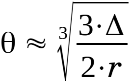 |
(2.3.14) |
Substitute eq. 2.3.9, eq. 2.3.10 og eq. 2.3.11 into eq. 2.3.8:
| |
(2.3.15) |
Cancel out the parentheses in eq. 2.3.15:
| |
(2.3.16) |
If or when the angle θ is very small the expressions with θ in highest orders will effectively be equal to zero. The expressions with θ4 and θ6 in eq. 2.3.16 will disappear and there remains:
| |
(2.3.17) |
That can be reduced to:
| |
(2.3.18) |
Substitute eq. 2.3.14 in eq. 2.3.18:
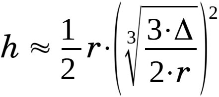 |
(2.3.19) |
Eq. 2.3.19 can then be written as:
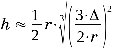 |
(2.3.20) |
Move radius "r" i eq. 2.3.20:
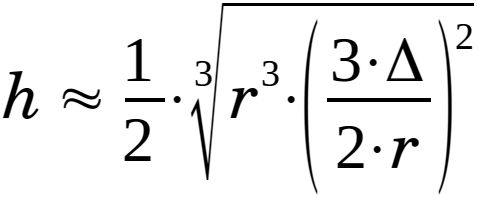 |
(2.3.21) |
Reduce and rearrange eq. 2.3.21 to arrive at the solution:
 |
(2.3.22) |
Strictly spoken isn't necessary first to evaluate the radius as shown in eq. 2.3.2 - you can substitute this equation into eq. 2.3.22:
 |
(2.3.23) |
Reduce and rearrange eq. 2.3.23 to arrive at an alternative formulation of the solution:
 |
(2.3.24) |
In the same way the angle can be found by substituting eq. 2.3.2 into eq. 2.3.14:
 |
(2.3.25) |
Reduce and rearrange eq. 2.3.25 to arrive at an alternative formulation for the angle:
 |
(2.3.26) |
The key-equations are:
| |
(2.3.2) | |
| |
(2.3.22) | |
| |
(2.3.14) |
Or:
| |
(2.3.24) | |
| |
(2.3.26) |
According to the formulation in § 2.1 and the assumptions in § 2.2:
Δ = 1 [m] ~ The elongation of the string.
c = 40 000 [km] = 40 000 000 [m] ~ The circumference of the earth.
When this value used in the analytical solution, first in eq. 2.3.2 and thereafter in eq. 2.3.22 the result becomes:
r = c/(2·π) = 40 000 000/(2·π)
≈
6 366 197 [m] (= 6 366 [km]).
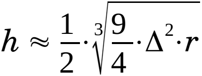
h
≈
½·
3√(9/4)·Δ2·r
≈
½·
3√(9/4)·12·6 366 197
≈
½·100·
3√(9/4)·6.366
≈
50·
3√14.324
≈
50·2.4286 ≈ 121 [m].
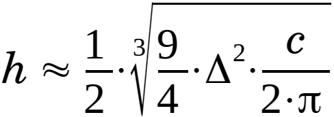
Or you can go directly to eq. 2.3.24, the result then becomes:
h ≈ ¼· 3√(9/π)·Δ2·c ≈ ¼· 3√(9/π)·12·40 000 000 ≈ ¼·100· 3√(9/π)·40 ≈ 25· 3√114.592 ≈ 25·4.8572 ≈ 121 [m].
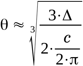
Is the angle θ very small as assumed? Use eq. 2.3.14:
θ ≈ 3√(3·Δ)/(2·r) ≈ 3√(3·1)/(2·6 366 197) ≈ (1/100)· 3√3/(2·6,366) ≈ (1/100)· 3√0.2356 ≈ 0.006176 [-] ≈ 0.354 [°].
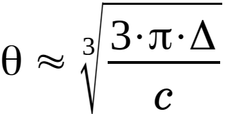
Or eq. 2.3.26:
θ ≈ 3√(3·π·Δ)/c ≈ 3√(3·π·1)/40 000 000 = (1/100)· 3√3·π/40 ≈ (1/100)· 3√0.2356 ≈ 0.006176 [-] ≈ 0.354 [°].
Less than one degree, that is really small.
You can very well arrive at the shown equations in an easier way, but must
then at the same time consider if θ is small and if the height is much
smaller than the radius of the earth, in other words:
θ ~ 0 and h << r. The shown projection in
fig. 2.7 can then be replaced by r/cos(θ) and eq. 2.3.7 becomes:
r + h = r/cos(θ)
If you compare the analytical equation, eq. 2.3.22 with a very precise numerical solution evaluated by iteration of equation 2.3.6 you can arrive at the relationship, shown below.
As a check of the iterated, numerical solution, the following expression is formulated, for height at very large elongations of the string:
| |
(2.5.1) |
If these 3 expressions for the height are plotted:
The result is:

Fig. 2.5.1: The height.
By looking at the curves, you must say, that the analytical solution for small elongations, in reality can't be distinguished from the exact solution up to around 3×1005, while the analytical solution for large elongations seems to be very accurate above approx. 3×1007. An evaluation of the deviation says that, for the analytical solution for small elongations, is an deviation of 2½ % at 23°, while it for the analytical solution for large elongations, is an deviation of 4½ % at 75°.
Ditto concerning the angles (here's the angle for the analytical solution for large angles constantly equal to 90°):

Fig. 2.5.2: The angle.
Some decades to each side of the desired 1 [m] elongation shows, how well the analytical solution fits:
| Δ [m] | h exact [m] | h analytical [m] | Relativd dev. [-] | Digits [-] |
|---|---|---|---|---|
| 1×10-06 | 0.01214295032 | 0.01214295031 | 5.72 E-10 | 9 |
| 1×10-03 | 1.2142951 | 1.2142950 | 5.72 E-08 | 7 |
| 1 | 121.4302 | 121.4295 | 5.72 E-06 | 5 |
| 1×1003 | 12150. | 12143. | 0.000572 | 3 |
| 1×1006 | 1283593. | 1214295. | 0.0540 | 2 |
|
|
|
|
|
To come...
|
|
|
|
|
| Overview |