
Claus Johansen, Sønderborg, Denmark, 2015-05-01 -> 2020-06-15
| Overview |
0) Contents:
3) A simple "text-book" example, given twist
4) Finding the (reaction) torque
5) Finding stress by given torque
7) Hollow sections, ex. 1, no symmetry used
8) Hollow sections, ex. 2, some symmetry used
 |
 |
 |
 |
Treating torsion as a thermal analogy can give tremendous reductions in problem size, in up to 3 steps:
The method is rarely described in FEA and if then often not in depth. E.g. twist pr. unit length used as input, but mostly a torque is known, not the twist - and in the cases where the twist is known, the corresponding torque will still be asked. How to take advantage of (multiple) symmetry? How to treat holes/hollow sections? These problems will be treated below.
Basis for § 3: "A simple "text-book" example, given twist" is an ANSYS® manual. All FEA are done in the ANSYS® FEA program - the "Classic/APDL" version.
The analytical values are all calculated by the formulas in: ROARK "Formulas for Stress and Strain".
| |
|
|
|
I first discovered the analogy in an ANSYS® manual, but it can also be found in various places on the Internet.
The shear stress under torsion can be computed as heat conduction, by simply swapping the letter designations. The reason is that it's basically the same differential equation that describes the phenomena:
| Heat conduction: |  |
(1) | |
| Torsion: | 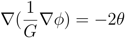 |
(2) |
The analogy is hereafter:
| Heat conduction | Torsion | ||||
|---|---|---|---|---|---|
 |
~ Temperature |  |
~ Stress function | ||
 |
~ (½) Heat generation pr. unit mass |  |
~ Twist pr. unit length | ||
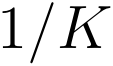 |
~ Reciprocal heat conductivity |  |
~ Shear modulus | ||
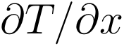 |
~ Temperature gradient x-dir. |  |
~ Shear stress yz | ||
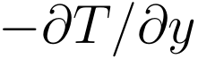 |
~ (negative) Temperature gradient y-dir. |  |
~ Shear stress xz | ||
The analogy covers also phenomena as: Electrostatics, membranes under pressure (soap film), seepage (permeability) through a porous medium, ideal flow (no rotation), etc.
|
|
|
|
|
The solution to this example is as I found it in an ANSYS® manual, but similar descriptions can be found various places on the Internet.
There are no difficulties in this example, only moderate hurdles can be to define the material property and find the twist pr. unit length when the total twist is known for the physical structure.
Below are the steps in a typical analysis: Geometry, material, element type, mesh, support, load and post-processing.
A cross-section in the bar is a solid quarter circle, radius ~ length of the straight sides is 10 mm. Here the geometry of the cross-section is represented by a plot of the area:
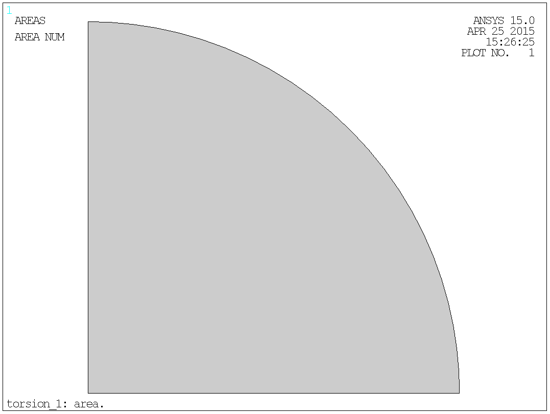
Fig. 3.1.1: Geometry.
The only material property needed is the heat conductivity. According to the analogy, as described in § 2, the heat conductivity "K" is simply the reciprocal of the shear modulus "G".
K = 1/G
If the specific value of the shear modulus isn't known the modulus of elasticity (Young's modulus) together with Poisson's ratio can be used as a basis. This will allow for consistent results if the results are compared with 3-D models.
G = E/(2(1+ν))
In a case with steel and units in N and mm, the values can be:
E = 205.e+3 [N/mm2].
ν = 0.3 [-].
G = E/(2(1+ν)) = 205.e+3/(2(1+0.3)) = 78846. [N/mm2].
K = 1/G = 1/78846 = 0.1268292683E-04
The element types shall preferably be a thermal 2-D element type. In ANSYS® these element types are no 55 or 77. No 55 is a triangular element and no 77 is quadrilateral.
In this example the area is meshed with the quadrilateral element, no 77 - ANSYS® does a good job in meshing with quad's in 2-D, so why not use this element where ever possible, as quad's in general are better/more efficient than triangles.
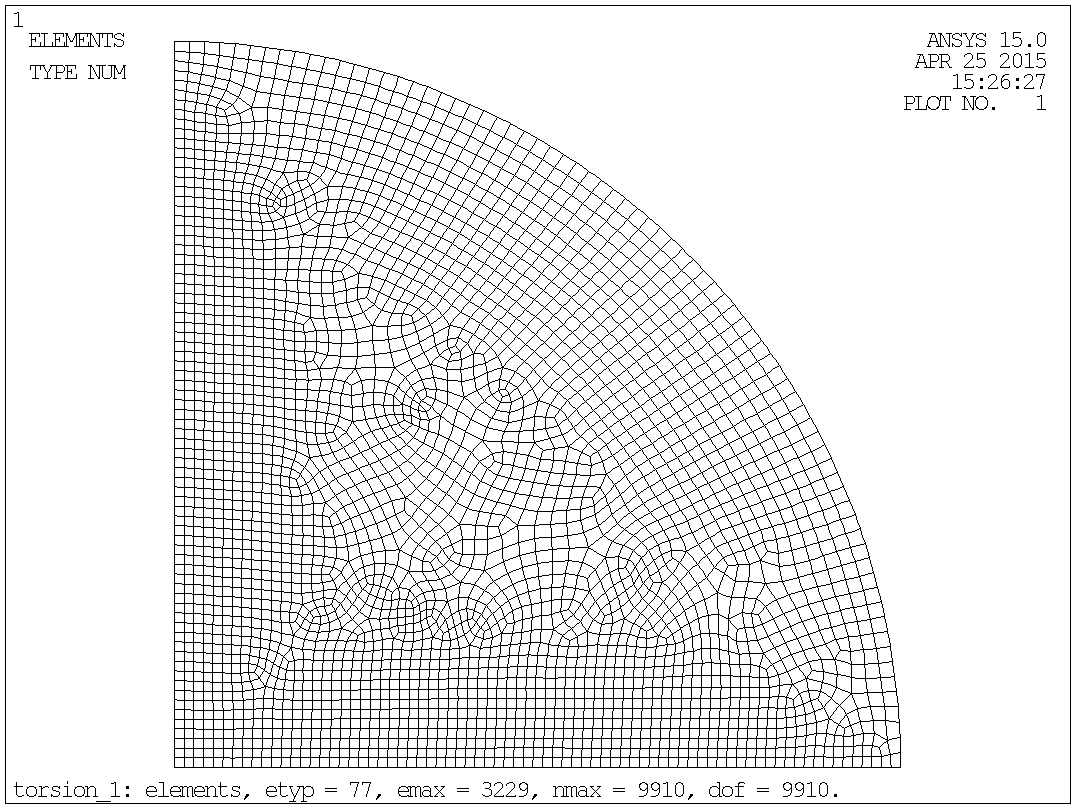
Fig. 3.4.1: Mesh.
The shown mesh, with element type 77, has 3229 elements, 9910 nodes and thereby also 9910 degrees of freedom. Though a relatively fine mesh still a small model.
The support consists simply of defining a temperature of zero along the outer boundary of the cross-section.
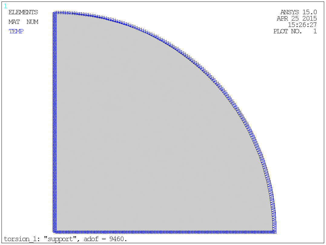
Fig. 3.5.1: Support.
The number of active degrees of freedom will be reduced moderately (to 9460) but it's probably without importance.
Assume a physical bar, with the cross-section described previously, and with a length of one meter and with a forced deflection of 10°.
Then the natural steps in finding the twist per unit length will be:
The forced defection in radians - convert the angular deflections in
degrees to radians:
θr = θ°·π/180 = 10·π/180 =
0.1745329252 [-].
The forced defection pr. unit length "twist" - The cross-section is
modelled in millimetres, so the length must be converted into mm and the
twist will be pr. mm:
θ = θr/1000 = 0.1745329252/1000 =
0.1745329252E-03 [1/mm].
Heat generation pr. unit mass - according to the analogy, as described in
§ 2, the heat generation pr. unit mass "q" is simply two times the
twist:
q = 2·θ = 2·0.1745329252E-03 = 0.3490658504E-03.
The heat generation is evenly distributed (constant) over cross-section:
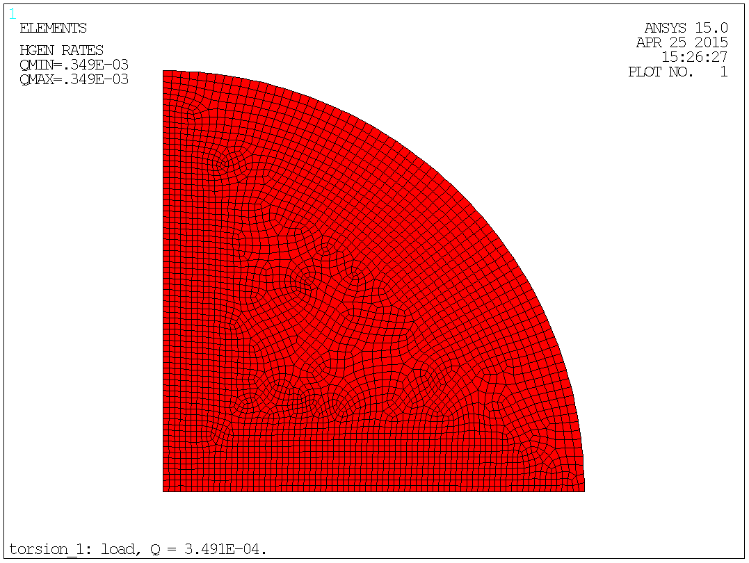
Fig. 3.6.1: Load.
A plot of the temperature will give the "shape" of the potential:
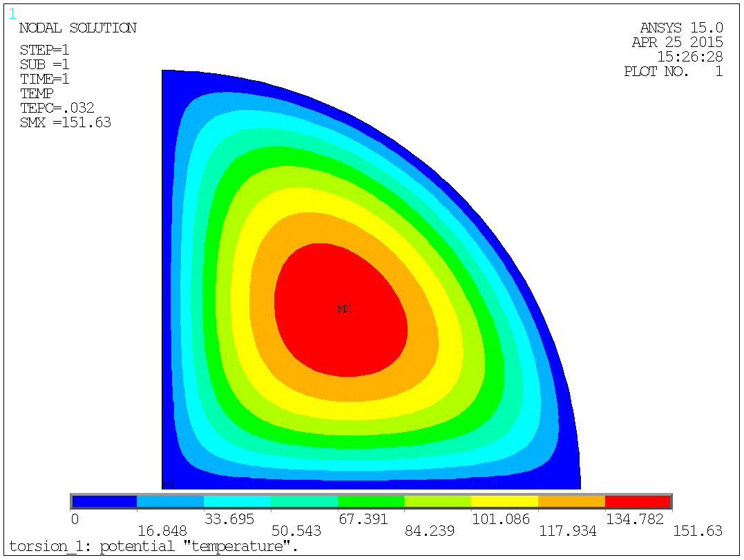
Fig. 3.7.1: The potential "temperature".
A plot of the thermal gradient will give the sear stress:
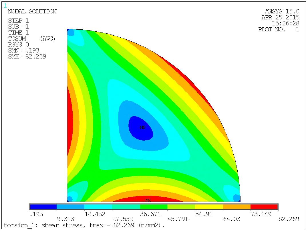
Fig. 3.7.2: The shear stress "thermal gradient".
The max shear stress can finally be converted to an equivalent stress by
the traditionally used relationship, in this case:
σ = τ·√3 = 82.26887512·√3 = 142.4938716
~ 142. [N/mm2].
|
|
|
|
|
During my long service as an engineer I never met a case, where stresses as a function of angular displacement "twist" only were asked. The problem was at least always followed by the question of the corresponding torque?
In a case as the text-book example in the previous section, where the geometry isn't naturally modelled around the geometric centre of the cross-section "CoG", there must be created a local coordinate system in this position.
In the Pre-processor, find the coordinates of the mass centre "CoG" by the commands:
asum ! sum area properties. *get,name,area,,cent,x $ xc= name ! x-pos. of mass centre. *get,name,area,,cent,y $ yc= name ! y-pos. of mass centre. |
Afterwards create a local coordinate system in this position - it's a large advantage if this local coordinate system is cylindrical, as shown here:
csys,0 $ dsys,0 local,11,1,xc,yc,0 ! local coord.sys. at CoG. csys,0 $ dsys,0 |
A plot with the local coordinate system indicated by the number "11":
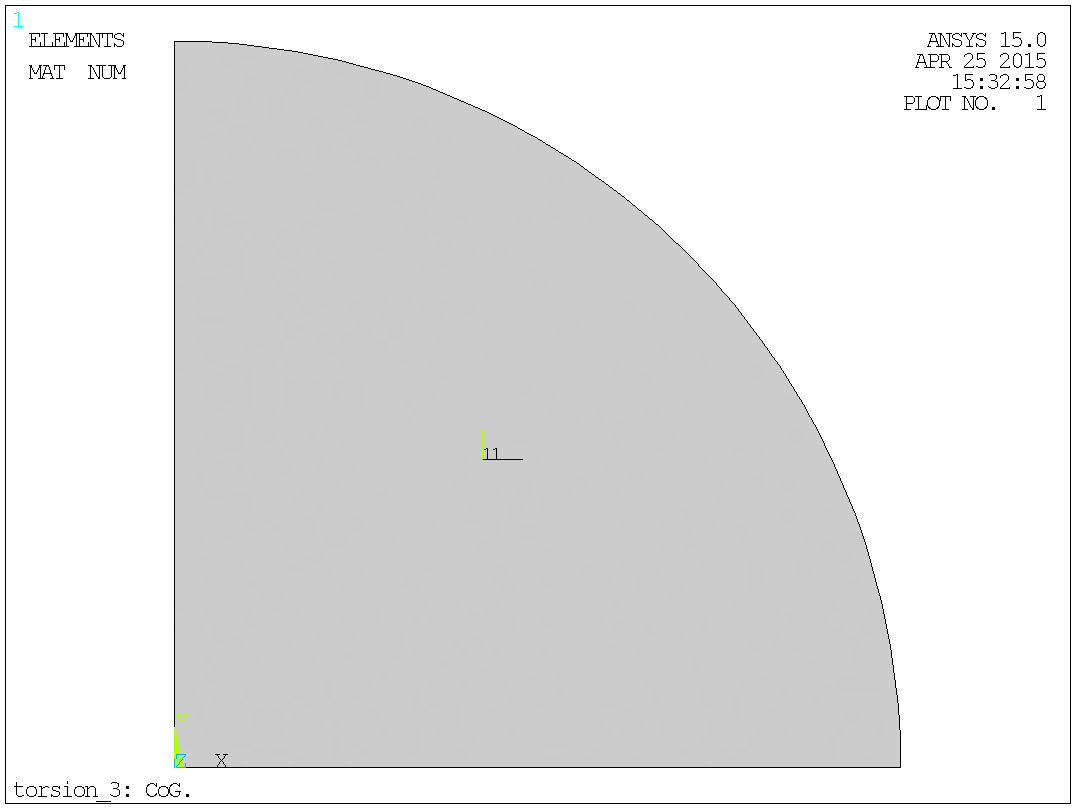
Fig. 4.1: The local coordinate system in CoG.
The torque is calculated with the facilities in the etable procedure, the principles sketched below:
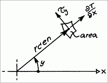
Fig. 4.2: Finding the torque.
The procedure that takes place in the commands below can be described as:
The commands are:
csys,11 $ dsys,11 $ rsys,11 ! cyl. coord. sys. at centre of mass. etable,rcen,cent,x ! element centre radius. etable,tauy,tg,x ! therm. gradient, radial component. etable,area,volu ! volume (depth == 1) eq. area. smult,df,area,tauy ! tangential force pr. element. smult,dt,df,rcen ! torque pr. element. ssum ! all etable values are summed up. *get,name,ssum,dt ! torque from sum to parametre "name". torq= -name ! torque in the shaft. |
The radial (X-dir.) thermal gradient corresponding to the tangential (Y-dir.) shear stress, that is used in the operations above, look like this:
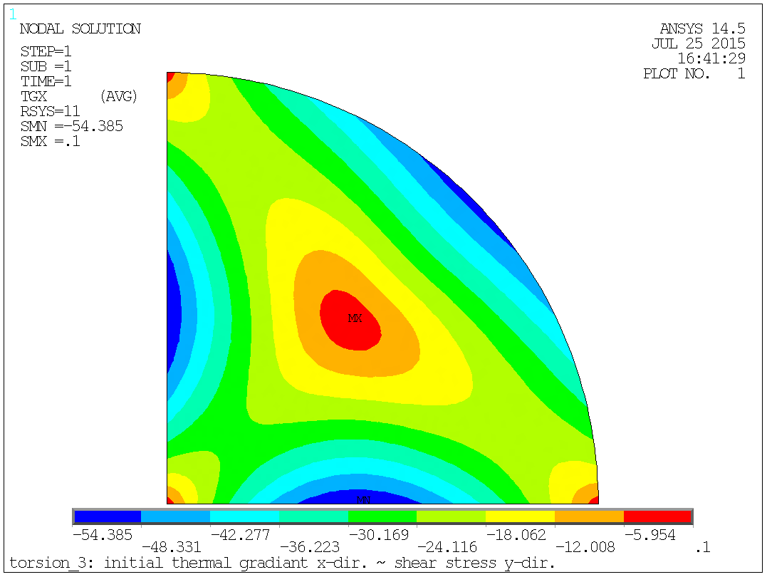
Fig. 4.3: Radial thermal gradient ~ tangential shear stress.
In the text-book example the torque that corresponds to the angular deflection of 10° for the 1000 [mm] long steel bar of a ¼ circular sector of radius 10 [mm] is calculated to [Nmm]:
PARAMETER TORQ = 11329.10468 |
The stiffness of the bar, or more precisely, the stiffness of a unit length of the bar, can now be calculated. The general formula is:
θr = (TL)/(KG)
Where:
T ~ Torque.
L ~ Length.
K ~ Stiffness.
G ~ Shear modulus.
By re-arranging the general formula K can be found to:
K = (TL)/(θrG) = T/(θG)
In this text-book example the stiffness "the effective torsional moment of inertia" of the bar of a ¼ circular sector of radius 10 [mm] is calculated to [mm4]:
PARAMETER KEFF = 823.2613159 |
This section "Finding the (reaction) torque" is essential for practical use of the analogy, and not only being of academic interest. It will also allow for a comparison with analytical formulas - stiffness and stresses at a given torque. I will below give an example of how the problem can be solved when the torque is known, and the stresses and deflection are the desired results. This represents to me a typical procedure in a torsional problem.
|
|
|
|
|
The geometry is as in the first example, § 3, and the procedures of finding the corresponding torque are as described in § 4, but as here the torque, not the twist, is known, it calls for a 2 step analysis. I'll describe it from the bottom again:
A cross-section in the bar is a solid quarter circle, radius ~ length of the straight sides is 10 mm. Here the geometry of the cross-section is represented by a plot of the area:
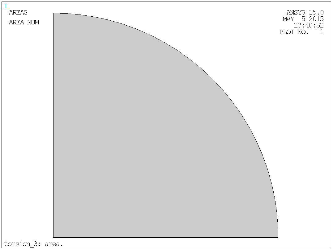
Fig. 5.1.1: Geometry.
The only material property needed is the heat conductivity. According to the analogy, as described in § 2, the heat conductivity "K" is simply the reciprocal of the shear modulus "G".
K = 1/G
If the specific value of the shear modulus isn't known the modulus of elasticity (Young's modulus) together with Poisson's ratio can be used as a basis. This will allow for consistent results if the results are compared with 3-D models.
G = E/(2(1+ν))
In a case with steel and units in N and mm, the values can be:
E = 205.e+3 [N/mm2].
ν = 0.3 [-].
G = E/(2(1+ν)) = (205.e+3)/(2(1+0.3)) = 78846. [N/mm2].
K = 1/G = 1/78846 = 0.1268292683E-04
Now if K is defined to this value in ANSYS®, the output shows:
PARAMETER K = 0.1268292683E-04 |
Then the command for the heat conductivity is:
mp,kxx,1,k |
And the output shows:
MATERIAL 1 KXX = 0.1268293E-04 |
In this example the area is meshed with the quadrilateral element, no 77 - ANSYS® does a good job in meshing with quad's in 2-D, so why not use this element where ever possible, as quad's in general are better/more efficient than triangles.

Fig. 5.3.1: Mesh.
The shown mesh, with element type 77, has 3229 elements, 9910 nodes and thereby also 9910 degrees of freedom. Though a relatively fine mesh still a small model.
Before leaving the pre-processor we can as well prepare load and torque calculation by issuing the "asum" command and extract polar moment of inertia (about CoG) and the position of CoG and place the coordinate system for (reaction) torque calculation here:
asum ! sum area properties. *get,name,area,,imc,z $ ip= name ! polar moment of inertia. *get,name,area,,cent,x $ xc= name ! x-pos. of mass centre. *get,name,area,,cent,y $ yc= name ! x-pos. of mass centre. |
And the output shows:
 PRINT GEOMETRY ITEMS ASSOCIATED WITH THE CURRENTLY SELECTED AREAS

 *** NOTE ***                            CP =       0.687   TIME= 22:12:13
 Density not associated with all selected areas.  Geometry items are
 based on a unit density.

  TOTAL NUMBER OF AREAS SELECTED =      1  (OUT OF      1 DEFINED)

  TOTAL SURFACE AREA OF ALL SELECTED AREAS =   78.540

  TOTAL VOLUME OF ALL SELECTED AREAS =   78.540

  CENTER OF MASS:  XC=  4.2441      YC=  4.2441      ZC=  0.0000

                    *** MOMENTS OF INERTIA ***
          (BASED ON A UNIT DENSITY AND A UNIT THICKNESS)

        ABOUT ORIGIN     ABOUT CENTER OF MASS    PRINCIPAL
    IXX =    1963.5            548.78            713.49
    IYY =    1963.5            548.78            384.07
    IZZ =    3927.0            1097.6            1097.6
    IXY =   -1250.0            164.71
    IYZ =    0.0000            0.0000
    IZX =    0.0000            0.0000

    PRINCIPAL ORIENTATION VECTORS (X,Y,Z):
      0.707  0.707  0.000   -0.707  0.707  0.000    0.000  0.000  1.000
      (THXY=   45.000  THYZ=    0.000  THZX=    0.000)

 *GET  NAME      FROM  AREA  ITEM=IMC  Z     VALUE=  1097.56639

 PARAMETER IP =     1097.566392

 *GET  NAME      FROM  AREA  ITEM=CENT X     VALUE=  4.24413177

 PARAMETER XC =     4.244131767

 *GET  NAME      FROM  AREA  ITEM=CENT Y     VALUE=  4.24413177

 PARAMETER YC =     4.244131767
|
Afterwards create a local coordinate system in this position - it's a large advantage if this local coordinate system is cylindrical, as shown here, the commands are:
csys,0 $ dsys,0 local,11,1,xc,yc,0 ! local coord.sys. at CoG. csys,0 $ dsys,0 |
And the output shows:
ACTIVE COORDINATE SYSTEM SET TO 0 (CARTESIAN) DISPLAY COORDINATE SYSTEM SET TO 0 (CARTESIAN) COORDINATE SYSTEM 11 DEFINITION. TYPE= 1 (CYLINDRICAL) XC,YC,ZC= 4.2441 4.2441 0.0000 ANGLES= 0.00 0.00 0.00 PARAMETERS= 1.000 1.000 ORIENTATION= 1.00 0.00 0.00 0.00 1.00 0.00 0.00 0.00 1.00 ACTIVE COORDINATE SYSTEM SET TO 11 (CYLINDRICAL) ACTIVE COORDINATE SYSTEM SET TO 0 (CARTESIAN) DISPLAY COORDINATE SYSTEM SET TO 0 (CARTESIAN) |
A plot with the local coordinate system indicated by the number "11":
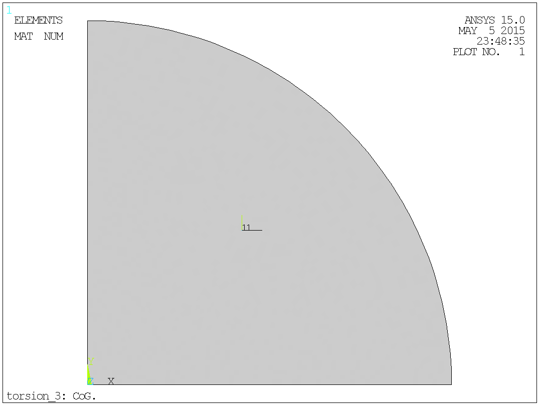
Fig. 5.4.1: The local coordinate system in CoG.
The support consists simply of defining a temperature of zero along the outer boundary of the cross-section.
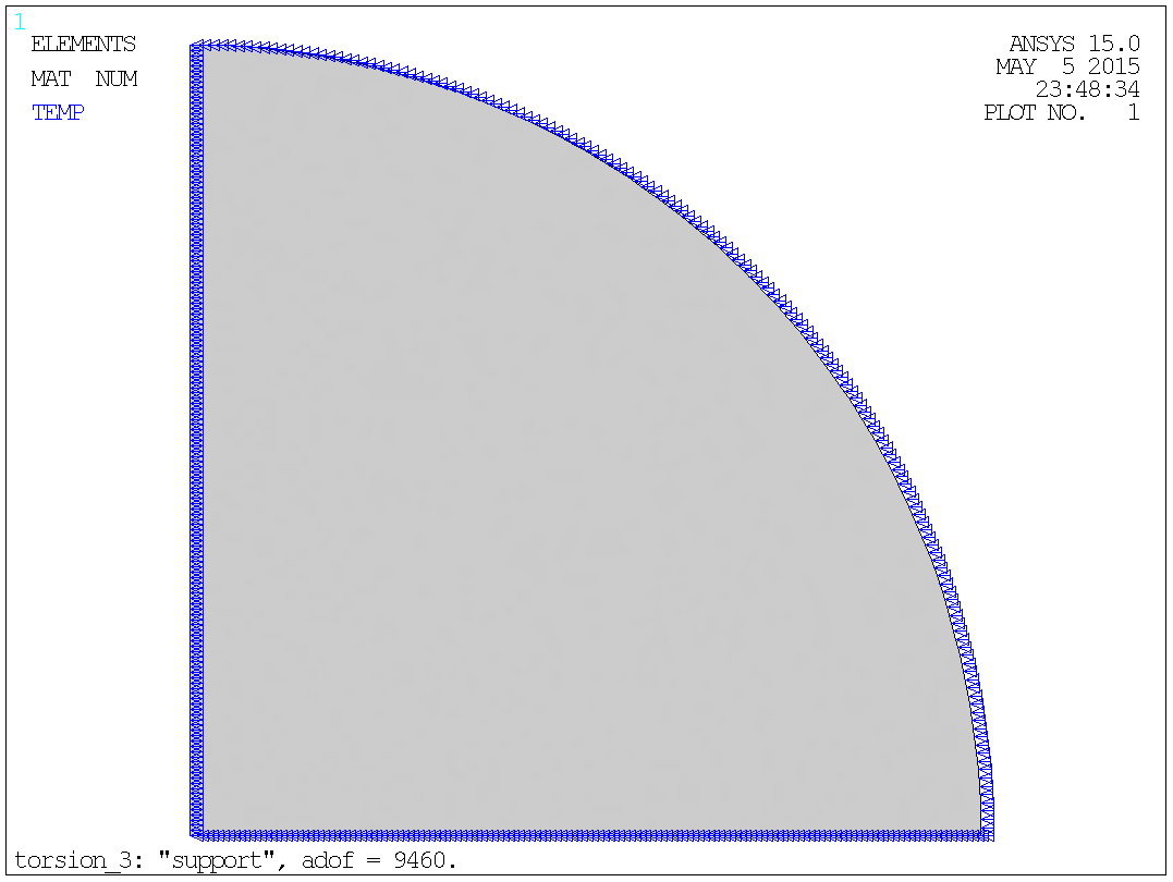
Fig. 5.5.1: Support.
The number of active degrees of freedom will be reduced moderately (to 9460) but it's probably without importance.
Let the torque be 1.e+4 = 10 000 [Nmm].
As the formula for angular deflection of a circular bar is:
θr = (TL)/(IpG)
Where:
T ~ Torque.
L ~ Length.
Ip ~ Polar moment of inertia.
G ~ Shear modulus.
Then the expression for angular deflection of a circular bar pr. unit length "twist" is:
θ = T/(IpG)
With:
T = 1.e+4 = 10000. [Nmm]. Given torque.
Ip = 1098. [mm4]. Polar moment of inertia as
described in § 5.4.
G = 78846. [N/mm2]. Shear modulus of steel as described in §
5.2.
The first guess on twist in the bar is the same as if the bar was circular - this is not the case, but it gives a first guess with some physical sense and a value that can have a reasonable size. Alternatively, a unit value could be used. In the end it should make no difference as the result of the initial load set will be scaled to obtain the correct final result.
The values below are only first guesses and will be designated by index 1.
The angular deflection of a circular steel bar pr. is unit length "twist" is:
θ1 = 10000/(1098·78846) = 0.1155549853E-03 [1/mm].
Heat generation pr. unit mass - according to the analogy, as described in § 2, the Heat generation pr. unit mass "q" is simply two times the twist:
q1 = 2·θ1 = 2·0.1155549853E-03 = 0.2311099705E-03
The heat generation is evenly distributed over cross-section:
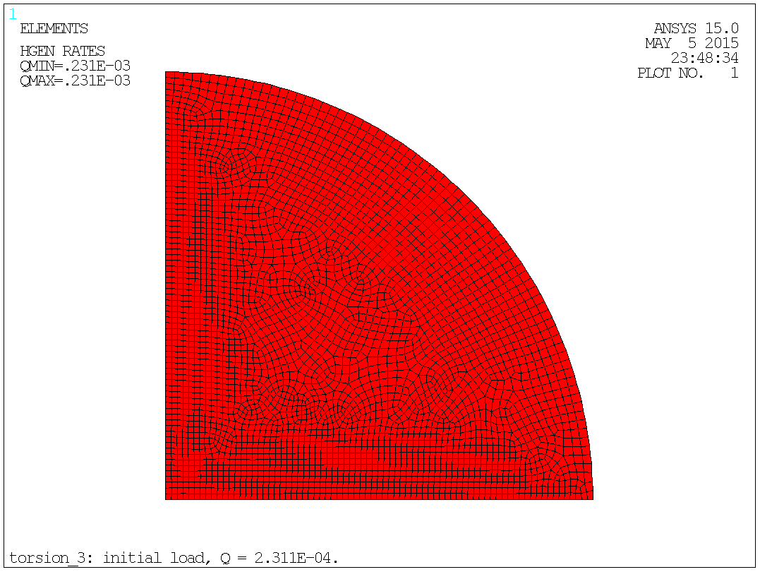
Fig. 5.6.1: Initial load.
The procedure is described in depth in § 4.
Solve the problem and go to the post-processor. The commands are:
csys,11 $ dsys,11 $ rsys,11 ! cyl. coord. sys. at centre of mass. etable,rcen,cent,x ! element centre radius. etable,tauy,tg,x ! therm. gradient, radial component. etable,area,volu ! volume (depth == 1) eq. area. smult,df,area,tauy ! tangential force pr. element. smult,dt,df,rcen ! torque pr. element. ssum ! all etable values are summed up. *get,name,ssum,dt ! torque from sum to parametre "name". torq1= -name ! torque in the shaft. |
The radial (X-dir.) thermal gradient corresponding to the tangential (Y-dir.) shear stress, that is used in the operations above, look like this:
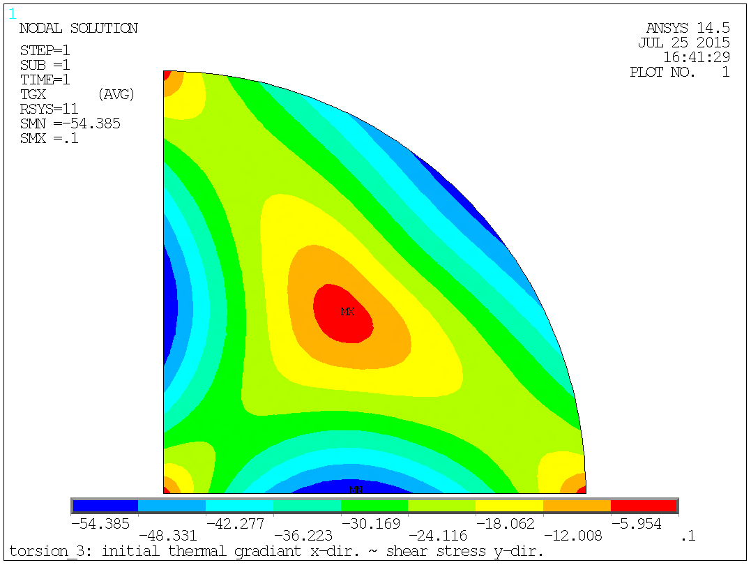
Fig. 5.7.1: Radial thermal gradient ~ tangential shear stress.
And the output shows:
ACTIVE COORDINATE SYSTEM SET TO 11 (CYLINDRICAL) DISPLAY COORDINATE SYSTEM SET TO 11 (CYLINDRICAL) RSYS KEY SET TO 11 USE COORDINATE SYSTEM 11 FOR SOLUTION RESULTS STORE RCEN FROM ITEM=CENT COMP=X FOR ALL SELECTED ELEMENTS STORE TAUY FROM ITEM=TG COMP=X FOR ALL SELECTED ELEMENTS STORE AREA FROM ITEM=VOLU FOR ALL SELECTED ELEMENTS OPERATION SMUL RESULT= DF OPERAND1= AREA OPERAND2= TAUY FACTOR1= 1.0000 FACTOR2= 1.0000 CONSTANT= 0.0000 OPERATION SMUL RESULT= DT OPERAND1= DF OPERAND2= RCEN FACTOR1= 1.0000 FACTOR2= 1.0000 CONSTANT= 0.0000 SUM ALL THE ACTIVE ENTRIES IN THE ELEMENT TABLE TABLE LABEL TOTAL RCEN 11400.5 TAUY -85239.0 AREA 78.5398 DF -2029.54 DT -7500.79 *GET NAME AS SSUM DT VALUE= -7500.788 PARAMETER TORQ1 = 7500.788304 |
With the initial guess on the twist we obtained a torque of 7 501 [Nmm] but 10 000 [Nmm] was desired.
Return to the solution-module and perform a new analysis with the final load.
To find the final twist the initial twist shall be scaled to compensate for the deviation in torque. Obtained 7 501 [Nmm], desired 10 000 [Nmm]:
θ2 = θ1·10000/7501 = 0.1155549853E-03·10000/7501 = 0.1540571212E-03 [1/mm].
Heat generation pr. unit mass - according to the analogy, as described in § 2, the Heat generation pr. unit mass "q" is simply two times the twist:
q2 = 2·θ2 = 2·0.1540571212E-03 = 0.3081142423E-03.
The heat generation is evenly distributed over cross-section:

Fig. 5.8.1: Final load.
The procedure is described in depth in § 4.
Solve the problem and go to the post-processor. The commands are:
csys,11 $ dsys,11 $ rsys,11 ! cyl. coord. sys. at centre of mass. etable,rcen,cent,x ! element centre radius. etable,tauy,tg,x ! therm. gradient, radial component. etable,area,volu ! volume (depth == 1) eq. area. smult,df,area,tauy ! tangential force pr. element. smult,dt,df,rcen ! torque pr. element. ssum ! all etable values are summed up. *get,name,ssum,dt ! torque from sum to parametre "name". torq2= -name ! torque in the shaft. |
The radial (X-dir.) thermal gradient corresponding to the tangential (Y-dir.) shear stress, that is used in the operations above, look like this:

Fig. 5.9.1: Radial thermal gradient ~ tangential shear stress.
And the output shows:
ACTIVE COORDINATE SYSTEM SET TO 11 (CYLINDRICAL) DISPLAY COORDINATE SYSTEM SET TO 11 (CYLINDRICAL) RSYS KEY SET TO 11 USE COORDINATE SYSTEM 11 FOR SOLUTION RESULTS STORE RCEN FROM ITEM=CENT COMP=X FOR ALL SELECTED ELEMENTS STORE TAUY FROM ITEM=TG COMP=X FOR ALL SELECTED ELEMENTS STORE AREA FROM ITEM=VOLU FOR ALL SELECTED ELEMENTS OPERATION SMUL RESULT= DF OPERAND1= AREA OPERAND2= TAUY FACTOR1= 1.0000 FACTOR2= 1.0000 CONSTANT= 0.0000 OPERATION SMUL RESULT= DT OPERAND1= DF OPERAND2= RCEN FACTOR1= 1.0000 FACTOR2= 1.0000 CONSTANT= 0.0000 SUM ALL THE ACTIVE ENTRIES IN THE ELEMENT TABLE TABLE LABEL TOTAL RCEN 11400.5 TAUY -113640. AREA 78.5398 DF -2705.77 DT -10000.0 *GET NAME AS SSUM DT VALUE= -10000.00 PARAMETER TORQ2 = 9999.999996 |
With the final guess on the twist we are spot-on with the obtained torque!
With the general formula for angular deflection of a bar:
θr = (TL)/(KG)
Where:
T ~ Torque.
L ~ Length.
K ~ Stiffness.
G ~ Shear modulus.
By re-arranging the general formula K can be found to:
K = (TL)/(θrG) = T/(θG)
In this example the stiffness "the effective torsional moment of inertia" of the bar of a ¼ circular sector of radius 10 [mm] is calculated to [mm4]:
K = T/(θG) = 10000/(0.1540571212E-03·78846) = 823.261 [mm4]
The analytical solution says K = 824.156 [mm4] a good agreement with the FEA value.
A plot of the temperature will give the "shape" of potential:
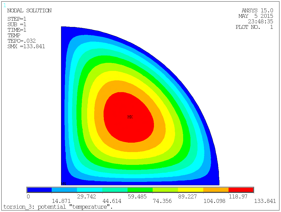
Fig. 5.11.1: The potential "temperature".
A plot of the thermal gradient will give the sear stress:
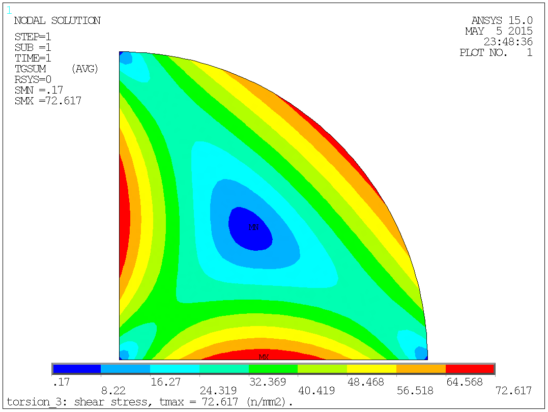
Fig. 5.11.2: The shear stress "thermal gradient".
Max shear stress can be read to: τ = 72.61728 ~ 73. [N/mm2].
The max shear stress can finally be converted to an equivalent stress by the
traditionally used relationship, in this case:
σ = τ·√3 = 72.61728·√3 = 125.7768168
~ 126. [N/mm2].
The analytical solution says τ = 72.6546181092 [N/mm2] a good agreement with the FEA value.
The iteration or better the scaling procedure can be shown as:
| Property | Symbol | Initial | Final | Formula |
|---|---|---|---|---|
| Initial stiffness | Ip | 1097.57 | ||
| Twist pr. unit length | θ | 0.115555 E-3 | 0.154057 E-3 | |
| Heat generation pr. unit mass | Q | 0.231110 E-3 | 0.308114 E-3 | |
| Torque | T | 7500.78 | 10000.0 | 10000.0 |
| Max shear stress | τ | 54.4687 | 72.6173 | 72.6546 |
| Stiffness | Keff | 823.261 | 823.261 | 824.156 |
|
|
|
|
|
To illustrate the method, I've chosen the somewhat special shape of a straight bar with a cross-section as an equilateral triangle, because there is a nice analytical solution to this problem.
Due to symmetry there is, 3 "teeth" (n=3), but a tooth also have a symmetry line giving an additional 2-fold symmetry. The FEA model will therefore only consist of: ½ "tooth", giving it a 3·2 = 6-fold symmetry:
Dimension: a = 10 [mm].
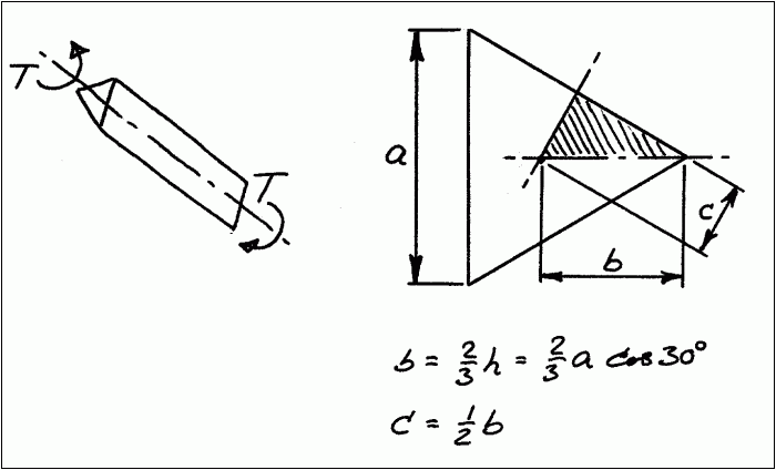
Fig. 6.1.1: Geometry.
A plot of the area as modelled in ANSYS®:
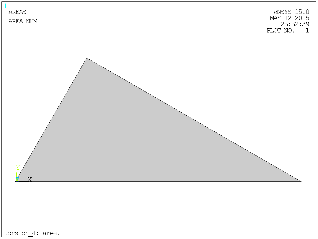
Fig. 6.1.2: Area.
The only material property needed is the heat conductivity. According to the analogy, as described in § 2, the heat conductivity "K" is simply the reciprocal of the shear modulus "G".
K = 1/G
If the specific value of the shear modulus isn't known the modulus of elasticity (Young's modulus) together with Poisson's ratio can be used as a basis. This will allow for consistent results if the results are compared with 3-D models.
G = E/(2(1+ν))
In a case with steel and units in N and mm, the values can be:
E = 205.e+3 [N/mm2].
ν = 0.3 [-].
G = E/(2(1+ν)) = (205.e+3)/(2(1+0.3)) = 78846. [N/mm2].
K = 1/G = 1/78846 = 0.1268292683E-04
Now if K is defined to this value in ANSYS®, so that the output shows:
PARAMETER K = 0.1268292683E-04 |
Then the command for the heat conductivity is:
mp,kxx,1,k |
And the output shows:
MATERIAL 1 KXX = 0.1268293E-04 |
In this example the area is meshed with the quadrilateral element, no 77 - ANSYS® does a good job in meshing with quad's in 2-D, so why not use this element where ever possible, as quad's in general are better/more efficient than triangles.
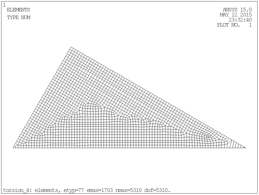
Fig. 6.3.1: Mesh.
The shown mesh, with element type 77, has 1703 elements, 5310 nodes and thereby also 5310 degrees of freedom. Though a relatively fine mesh still a small model.
Before leaving the pre-processor we can as well prepare load and torque calculation by issuing the "asum" command and extract polar moment of inertia. It's natural, and assumed here, that the geometry is modelled so, that the centre of the full geometry is positioned in the centre of the global coordinate system(s). "fold" = 6:
asum ! sum area properties. *get,name,area,,ior,z ! 1/6 polar moment of inertia. ip= name*fold ! total polar moment of inertia. |
And the output shows:
 PRINT GEOMETRY ITEMS ASSOCIATED WITH THE CURRENTLY SELECTED AREAS

 *** NOTE ***                            CP =       0.688   TIME= 23:32:39
 Density not associated with all selected areas.  Geometry items are
 based on a unit density.

   TOTAL NUMBER OF AREAS SELECTED =      1  (OUT OF      1 DEFINED)

   TOTAL SURFACE AREA OF ALL SELECTED AREAS =   7.2169

   TOTAL VOLUME OF ALL SELECTED AREAS =   7.2169

   CENTER OF MASS:  XC=  2.4056      YC= 0.83333      ZC=  0.0000

                     *** MOMENTS OF INERTIA ***
           (BASED ON A UNIT DENSITY AND A UNIT THICKNESS)

         ABOUT ORIGIN     ABOUT CENTER OF MASS    PRINCIPAL
     IXX =    7.5176            2.5059            2.2624
     IYY =    52.623            10.859            11.102
     IZZ =    60.141            13.365            13.365
     IXY =   -13.021            1.4468
     IYZ =    0.0000            0.0000
     IZX =    0.0000            0.0000

     PRINCIPAL ORIENTATION VECTORS (X,Y,Z):
       0.986 -0.166  0.000    0.166  0.986  0.000    0.000  0.000  1.000
       (THXY=   -9.553  THYZ=    0.000  THZX=    0.000)

 *GET  NAME      FROM  AREA  ITEM=IOR  Z     VALUE=  60.1406530

 PARAMETER IP =     360.8439182
|
The support consists simply of defining a temperature of zero along the outer boundary of the cross-section. There is only this one line on an outer boundary, the two other lines are internal symmetry lines:
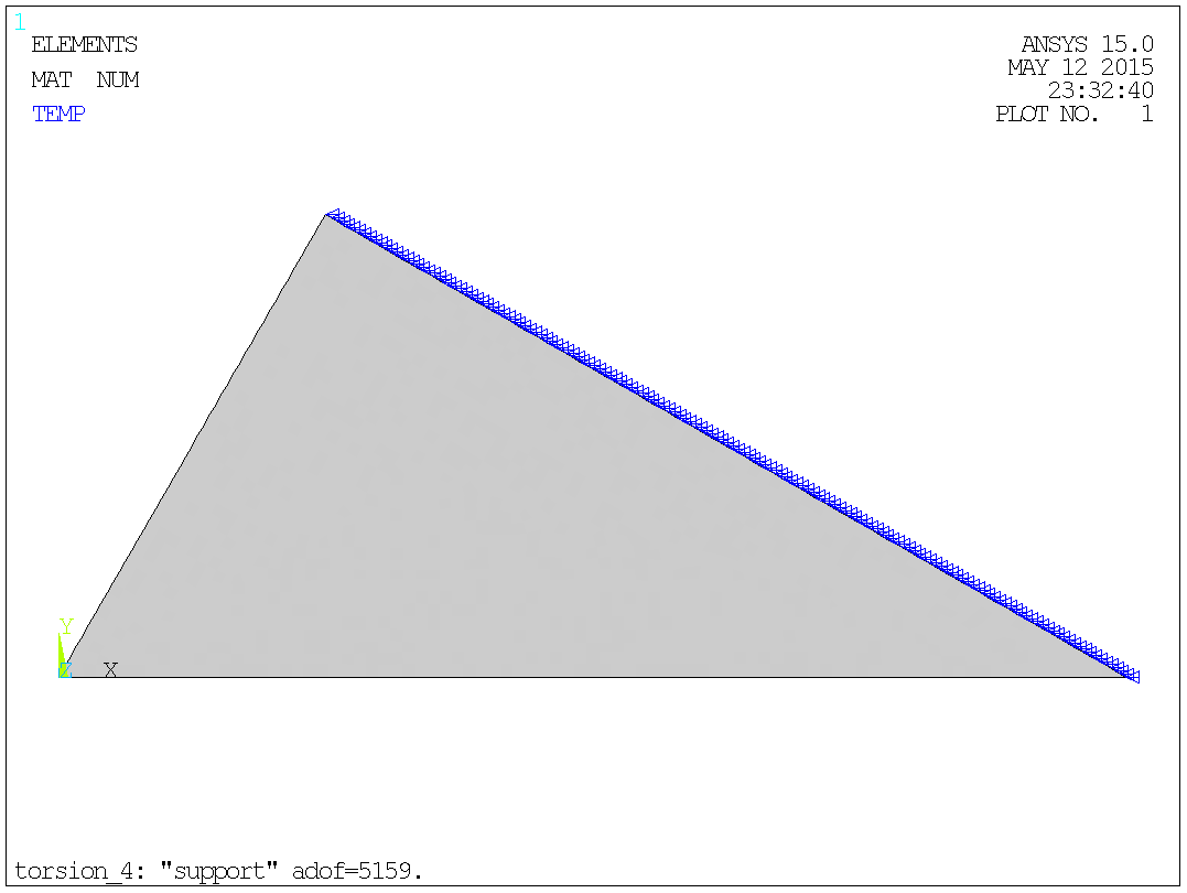
Fig. 6.5.1: Support.
The number of active degrees of freedom will be reduced moderately (to 5159) but it's probably without importance.
Let the torque be 1.e+4 = 10 000 [Nmm].
As the formula for angular deflection of a circular bar is:
θr = (TL)/(IpG)
Where:
T ~ Torque.
L ~ Length.
Ip ~ Polar moment of inertia.
G ~ Shear modulus.
Then the expression for angular deflection of a circular bar pr. is unit length "twist" is:
θ = T/(IpG)
With:
T = 1.e+4 = 10000. [Nmm]. Given torque.
Ip = 360.844 [mm4]. Polar moment of inertia as
described in § 6.4.
G = 78846. [N/mm2]. Shear modulus of steel as described in §
6.2.
The first guess on twist in the bar is the same as if the bar was circular - this is not the case, but it gives a first guess with some physical sense and a value that can have a reasonable size. Alternatively, a unit value could be used. In the end it should make no difference as the result of the initial load set will be scaled to obtain the correct final result.
The values below are only first guesses and will be designated by index 1.
The angular deflection of a circular steel bar pr. is unit length "twist" is:
θ1 = 10000/(360.844·78846) = 0.3514795785E-03 [1/mm].
Heat generation pr. unit mass - according to the analogy, as described in § 2, the Heat generation pr. unit mass "q" is simply two times the twist:
q1 = 2·θ1 = 2·0.3514795785E-03 = 0.7029591570E-03
The heat generation is evenly distributed over cross-section:
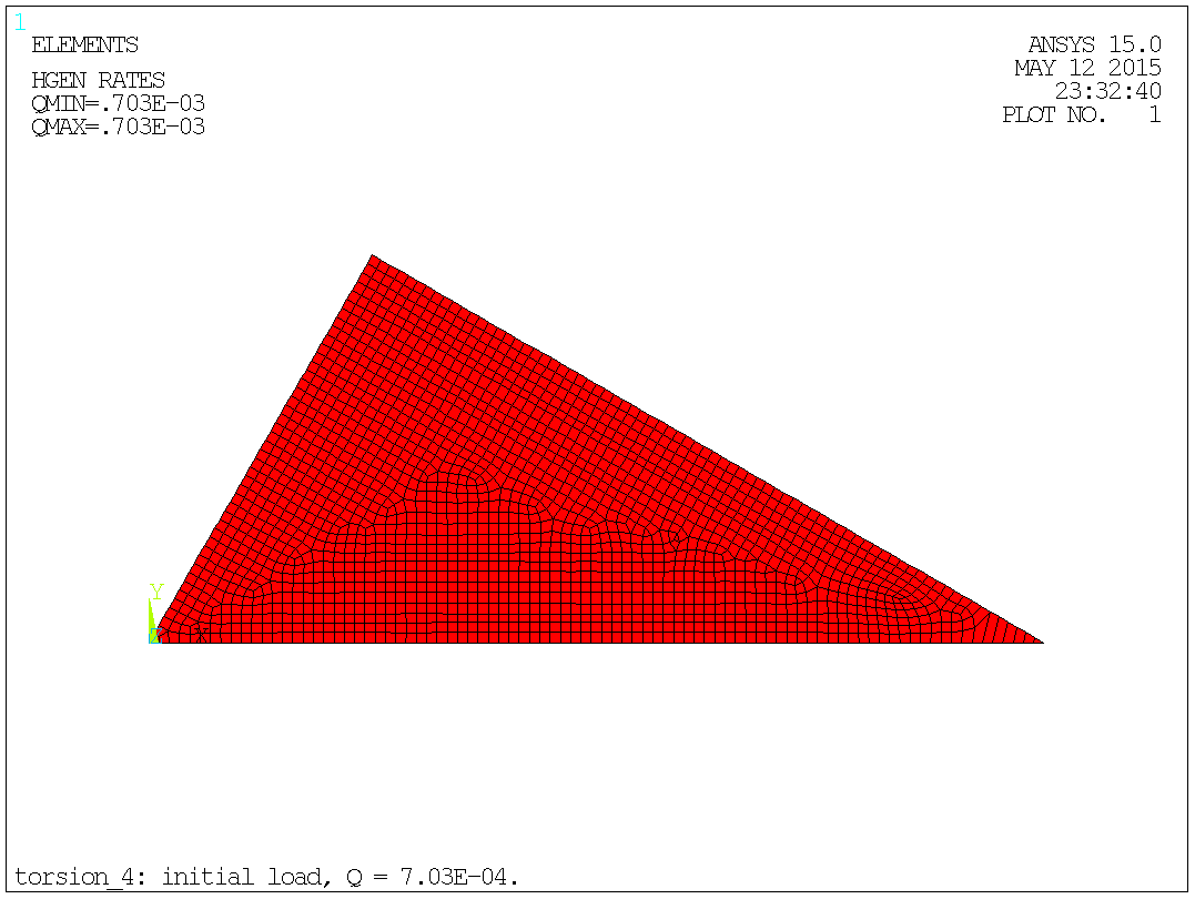
Fig. 6.6.1: Initial load.
The procedure is described in depth in § 4. The coordinate system for calculations is now no 1 - global cylindrical coordinate system in the centre of the full geometry.
Solve the problem and go to the post-processor. The commands are (fold = 6):
csys,1 $ dsys,1 $ rsys,1 ! cyl. coord. sys. at centre. etable,rcen,cent,x ! element centre radius. etable,tauy,tg,x ! therm. gradient, radial component. etable,area,volu ! volue (depth == 1) eq. area. smult,df,area,tauy ! tangential force pr. element. smult,dt,df,rcen ! torque pr. element. ssum ! all etable values are summed up. *get,name,ssum,dt ! torque from sum into parametre "name". torq1= -name*fold ! torque for the whole shaft. |
The radial (X-dir.) thermal gradient corresponding to the tangential (Y-dir.) shear stress, that is used in the operations above, look like this:
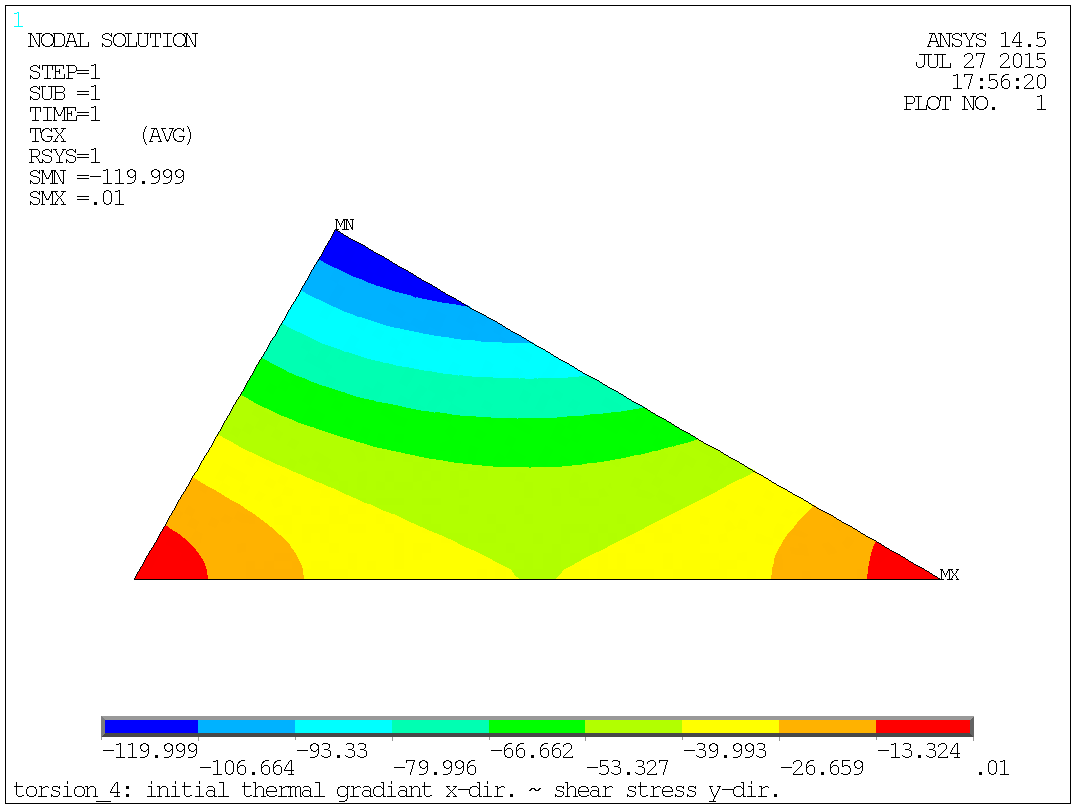
Fig. 6.7.1: Radial thermal gradient ~ tangential shear stress.
And the output shows:
ACTIVE COORDINATE SYSTEM SET TO 1 (CYLINDRICAL) Z- CYL. AXIS DISPLAY COORDINATE SYSTEM SET TO 1 (CYLINDRICAL) RSYS KEY SET TO 1 USE COORDINATE SYSTEM 1 FOR SOLUTION RESULTS STORE RCEN FROM ITEM=CENT COMP=X FOR ALL SELECTED ELEMENTS STORE TAUY FROM ITEM=TG COMP=X FOR ALL SELECTED ELEMENTS STORE AREA FROM ITEM=VOLU FOR ALL SELECTED ELEMENTS OPERATION SMUL RESULT= DF OPERAND1= AREA OPERAND2= TAUY FACTOR1= 1.0000 FACTOR2= 1.0000 CONSTANT= 0.0000 OPERATION SMUL RESULT= DT OPERAND1= DF OPERAND2= RCEN FACTOR1= 1.0000 FACTOR2= 1.0000 CONSTANT= 0.0000 SUM ALL THE ACTIVE ENTRIES IN THE ELEMENT TABLE TABLE LABEL TOTAL RCEN 4528.24 TAUY -87181.9 AREA 7.21688 DF -372.637 DT -1000.08 *GET NAME AS SSUM DT VALUE= -1000.077 PARAMETER TORQ1 = 6000.461938 |
With the initial guess on the twist we obtained a torque of 6 000 [Nmm] but 10 000 [Nmm] was desired.
Return to the solution-module and perform a new analysis with the final load.
To find the final twist the initial twist shall be scaled to compensate for the deviation in torque. Obtained 6 000 [Nmm], desired 10 000 [Nmm]:
θ2 = θ1·10000/6 000 = 0.3514795785E-03·10000/6000 = 0.5857542005E-03 [1/mm].
Heat generation pr. unit mass - according to the analogy, as described in § 2, the Heat generation pr. unit mass "q" is simply two times the twist:
q2 = 2·θ2 = 2·0.5857542005E-03 = 0.1171508401E-02.
The heat generation is evenly distributed over cross-section:
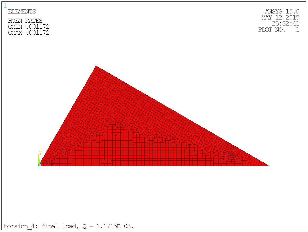
Fig. 6.8.1: Final load.
The procedure is described in depth in § 4.
Solve the problem and go to the post-processor. The commands are (fold = 6 ):
csys,1 $ dsys,1 $ rsys,1 ! cyl. coord. sys. at centre. etable,rcen,cent,x ! element centre radius. etable,tauy,tg,x ! therm. gradient, radial component. etable,area,volu ! volue (depth == 1) eq. area. smult,df,area,tauy ! tangential force pr. element. smult,dm,df,rcen ! torque pr. element. ssum ! all etable values are summed up. *get,name,ssum,dt ! torque from sum into parametre "name". torq2= -name*fold ! torque for the whole shaft. |
The radial (X-dir.) thermal gradient corresponding to the tangential (Y-dir.) shear stress, that is used in the operations above, look like this:
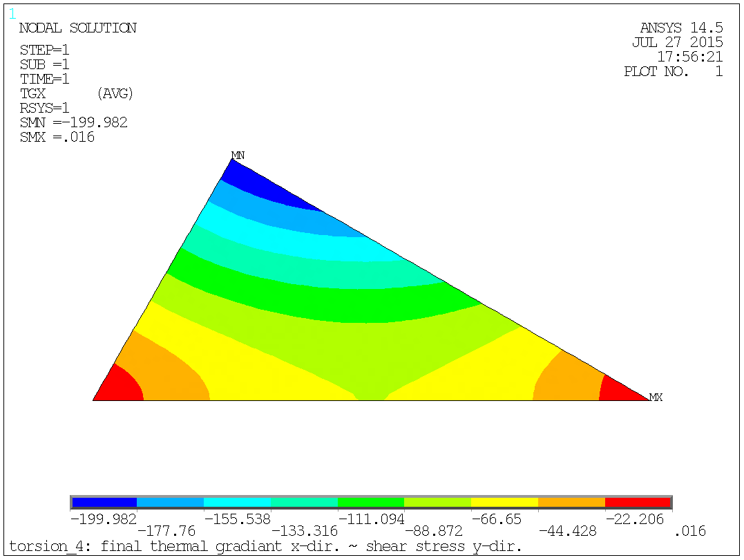
Fig. 6.9.1: Radial thermal gradient ~ tangential shear stress.
And the output shows:
ACTIVE COORDINATE SYSTEM SET TO 1 (CYLINDRICAL) Z- CYL. AXIS DISPLAY COORDINATE SYSTEM SET TO 1 (CYLINDRICAL) RSYS KEY SET TO 1 USE COORDINATE SYSTEM 1 FOR SOLUTION RESULTS STORE RCEN FROM ITEM=CENT COMP=X FOR ALL SELECTED ELEMENTS STORE TAUY FROM ITEM=TG COMP=X FOR ALL SELECTED ELEMENTS STORE AREA FROM ITEM=VOLU FOR ALL SELECTED ELEMENTS OPERATION SMUL RESULT= DF OPERAND1= AREA OPERAND2= TAUY FACTOR1= 1.0000 FACTOR2= 1.0000 CONSTANT= 0.0000 OPERATION SMUL RESULT= DT OPERAND1= DF OPERAND2= RCEN FACTOR1= 1.0000 FACTOR2= 1.0000 CONSTANT= 0.0000 SUM ALL THE ACTIVE ENTRIES IN THE ELEMENT TABLE TABLE LABEL TOTAL RCEN 4528.24 TAUY -145292. AREA 7.21688 DF -621.013 DT -1666.67 *GET NAME AS SSUM DT VALUE= -1666.667 PARAMETER TORQ2 = 9999.999997 |
With the final guess on the twist we are spot-on with the obtained torque!
With the general formula for angular deflection of a bar:
θr = (TL)/(KG)
Where:
T ~ Torque.
L ~ Length.
K ~ Stiffness.
G ~ Shear modulus.
By re-arranging the general formula K can be found to:
K = (TL)/(θrG) = T/(θG)
In this example the stiffness "the effective torsional moment of inertia" of the bar of a cross-section as an equilateral triangle of side length of 10 [mm] is calculated to [mm4]:
K = T/(θG) = 10000/(0.5857542005E-03·78846) = 216.523 [mm4]
The analytical solution says K = 216.506 [mm4] a very good agreement with the FEA value.
A plot of the temperature will give the "shape" of potential:
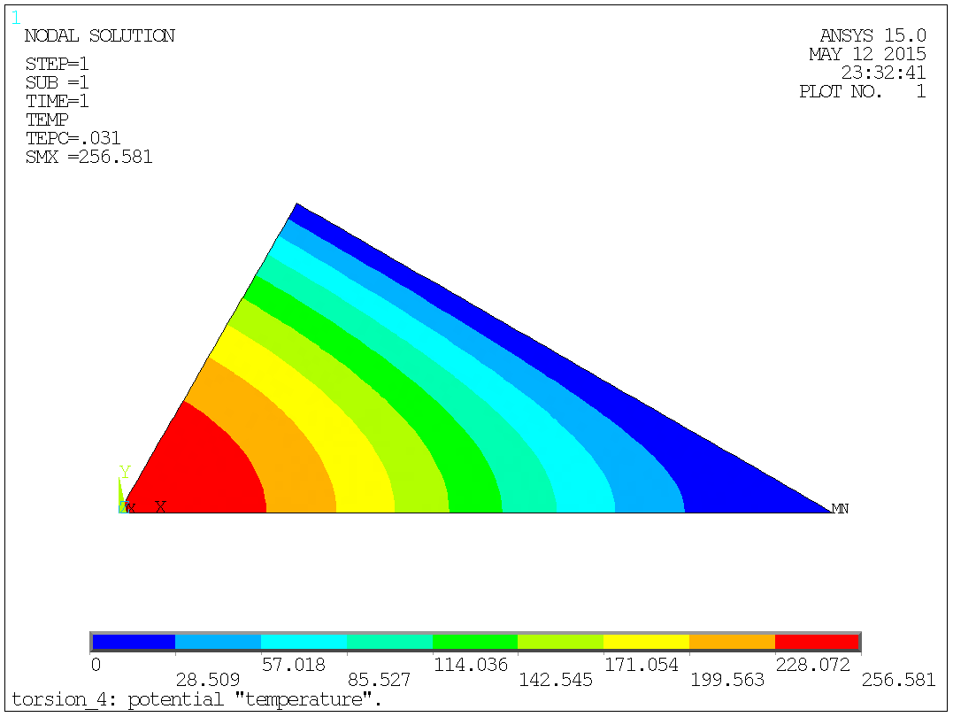
Fig. 6.11.1: The potential "temperature".
A plot of the thermal gradient will give the sear stress:
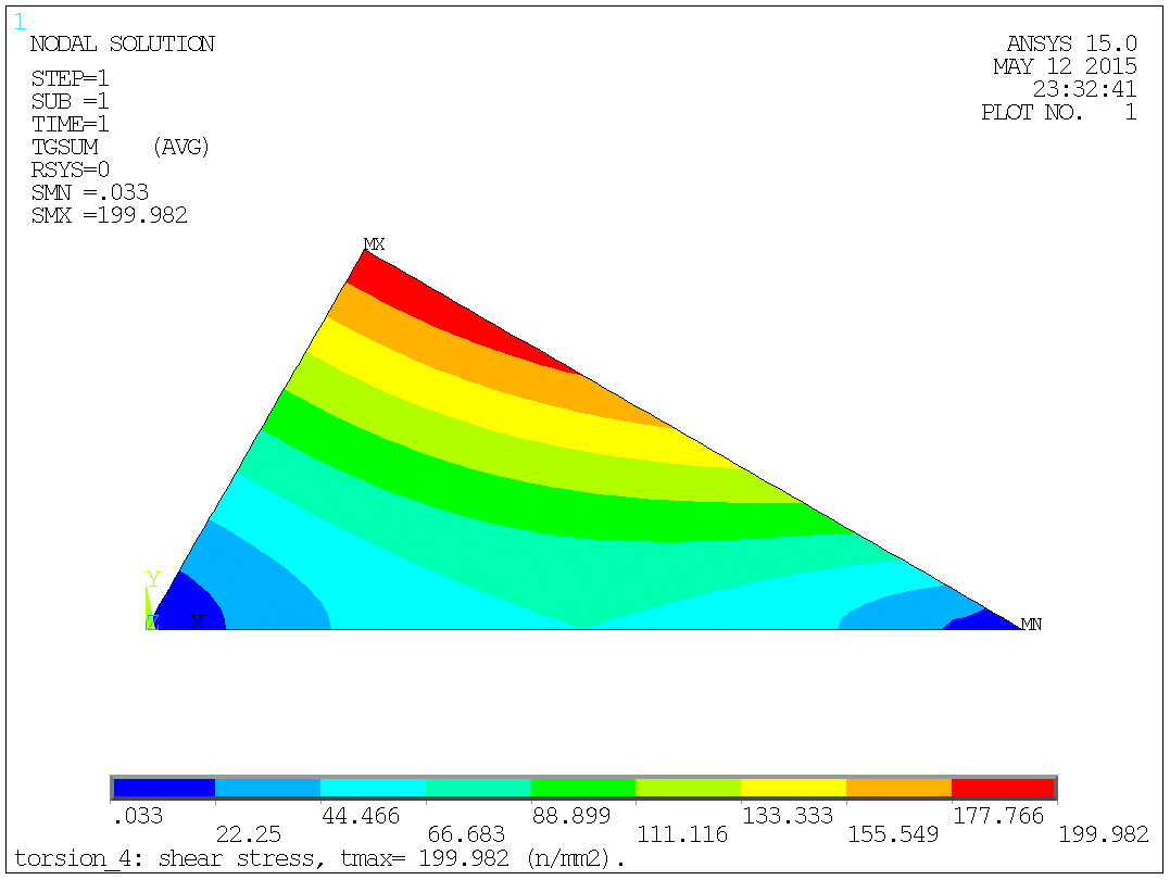
Fig. 6.11.2: The shear stress "thermal gradient".
Max shear stress can be read to: τ = 199.9824 ~ 200. [N/mm2].
The max shear stress can finally be converted to an equivalent stress by
the traditionally used relationship, in this case:
σ = τ·√3 = 199.9824·√3 = 346.3797036
~ 346. [N/mm2].
The analytical solution says τ = 200. [N/mm2] a good agreement with the FEA value.
The stress plot can finally be graphically expanded in ANSYS®, the command used here is:
/expand,fold,polar,half,0,(360/fold),0 |
The stress plot of the full cross-section of the shaft will then look like:
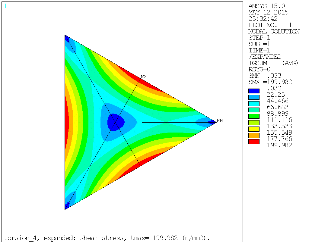
Fig. 6.11.3: The shear stress, full cross-section "thermal gradient".
The iteration or better the scaling procedure can be shown as:
| Property | Symbol | Initial | Final | Formula |
|---|---|---|---|---|
| Initial stiffness | Ip | 360.844 | ||
| Twist pr. unit length | θ | 0.351480 E-03 | 0.585754 E-03 | |
| Heat generation pr. unit mass | Q | 0.702959 E-03 | 0.117151 E-02 | |
| Torque | T | 6000.46 | 10000.0 | 10000.0 |
| Max shear stress | τ | 119.999 | 199.982 | 200.000 |
| Stiffness | Keff | 216.523 | 216.523 | 216.506 |
|
|
|
|
|
To illustrate the method, I've chosen the somewhat special shape of a straight bar with a cross-section as circle with an eccentric circular hole, because there is a nice analytical solution to this problem. The symmetry isn't used to reduce the problem size.
The diameter of the shaft is 4 [mm] and the hole has a diameter of 2 [mm]. The hole is 0.5 [mm] eccentric to the centre of the shaft.
A plot of the areas as modelled in ANSYS®. Both the solid part of the shaft and the hole are modelled - the hole must be meshed too, so it needs to be modelled too (argument in § 7.5):
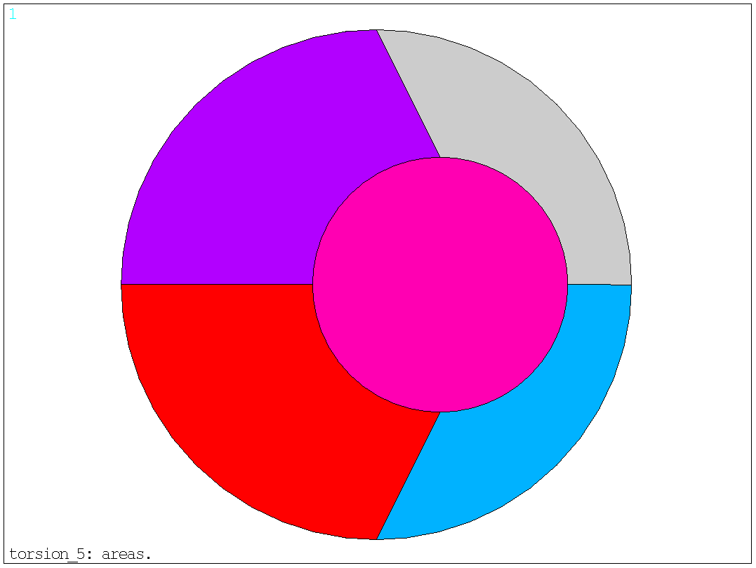
Fig. 7.1.1: Areas.
The only material property needed is the heat conductivity. According to the analogy, as described in § 2, the heat conductivity "K" is simply the reciprocal of the shear modulus "G".
K = 1/G
If the specific value of the shear modulus isn't known the modulus of elasticity (Young's modulus) together with Poisson's ratio can be used as a basis. This will allow for consistent results if the results are compared with 3-D models.
G = E/(2(1+ν))
In a case with steel and units in N and mm, the values can be:
E = 205.e+3 [N/mm2].
ν = 0.3 [-].
G = E/(2(1+ν)) = (205.e+3)/(2(1+0.3)) = 78846. [N/mm2].
K = 1/G = 1/78846 = 0.1268292683E-04
Now if K is defined to this value in ANSYS®, so that the output shows:
PARAMETER K = 0.1268292683E-04 |
Then the command for the heat conductivity is:
mp,kxx,1,k |
And the output shows:
MATERIAL 1 KXX = 0.1268293E-04 |
In this example the areas are meshed with the quadrilateral element, no 77 - ANSYS® does a good job in meshing with quad's in 2-D, so why not use this element where ever possible, as quad's in general are better/more efficient than triangles. The hole is modelled too, and it must also be meshed (argument in § 7.5):
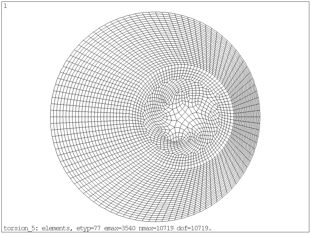
Fig. 7.3.1: Mesh.
The shown mesh, with element type 77, has 3540 elements, 10719 nodes and thereby also 10719 degrees of freedom. Though a relatively fine mesh still a small model.
Before leaving the pre-processor we can as well prepare load and torque calculation by issuing the "asum" command and extract polar moment of inertia (about CoG) and the position of CoG and place the coordinate system for (reaction) torque calculation here. Only the solid part of the shaft is analysed here:
asel,s,area,,1,4 asum ! sum area properties. *get,name,area,,imc,z $ ip= name ! polar moment of inertia. *get,name,area,,cent,x $ xc= name ! x-pos. of mass centre. |
And the output shows:
 PRINT GEOMETRY ITEMS ASSOCIATED WITH THE CURRENTLY SELECTED AREAS

 *** NOTE ***                            CP =       0.687   TIME= 22:12:13
 Density not associated with all selected areas.  Geometry items are
 based on a unit density.

   TOTAL NUMBER OF AREAS SELECTED =      4  (OUT OF      5 DEFINED)

   TOTAL SURFACE AREA OF ALL SELECTED AREAS =   9.4248

   TOTAL VOLUME OF ALL SELECTED AREAS =   9.4248

   CENTER OF MASS:  XC=-0.16667      YC=-0.91025E-09  ZC=  0.0000

                     *** MOMENTS OF INERTIA ***
           (BASED ON A UNIT DENSITY AND A UNIT THICKNESS)

         ABOUT ORIGIN     ABOUT CENTER OF MASS    PRINCIPAL
     IXX =    11.781            11.781            11.781
     IYY =    10.996            10.734            10.734
     IZZ =    22.776            22.515            22.515
     IXY =   0.58166E-05       0.58180E-05
     IYZ =    0.0000            0.0000
     IZX =    0.0000            0.0000

     PRINCIPAL ORIENTATION VECTORS (X,Y,Z):
       1.000  0.000  0.000    0.000  1.000  0.000    0.000  0.000  1.000
       (THXY=    0.000  THYZ=    0.000  THZX=    0.000)

 *GET  NAME      FROM  AREA  ITEM=IMC  Z     VALUE=  22.5146694

 PARAMETER IP =     22.51466935

 *GET  NAME      FROM  AREA  ITEM=CENT X     VALUE=-0.166666669

 PARAMETER XC =   -0.1666666686
|
Afterwards create a local coordinate system in this position - it's a large advantage if this local coordinate system is cylindrical, as shown here, the commands are:
csys,0 $ dsys,0 local,12,1,xc,0,0 ! local coord.sys. at CoG. csys,0 $ dsys,0 |
And the output shows:
ACTIVE COORDINATE SYSTEM SET TO 0 (CARTESIAN) DISPLAY COORDINATE SYSTEM SET TO 0 (CARTESIAN) COORDINATE SYSTEM 12 DEFINITION. TYPE= 1 (CYLINDRICAL) XC,YC,ZC=-0.16667 0.0000 0.0000 ANGLES= 0.00 0.00 0.00 PARAMETERS= 1.000 1.000 ORIENTATION= 1.00 0.00 0.00 0.00 1.00 0.00 0.00 0.00 1.00 ACTIVE COORDINATE SYSTEM SET TO 12 (CYLINDRICAL) ACTIVE COORDINATE SYSTEM SET TO 0 (CARTESIAN) |
The centre of the (outer) shaft circle is the global coord.sys. marked by "XYZ". The centre of the hole is the local coord.sys. no 11, to the right. The CoG of (the solid part of) the shaft is the local coord.sys. no 12, to the left:
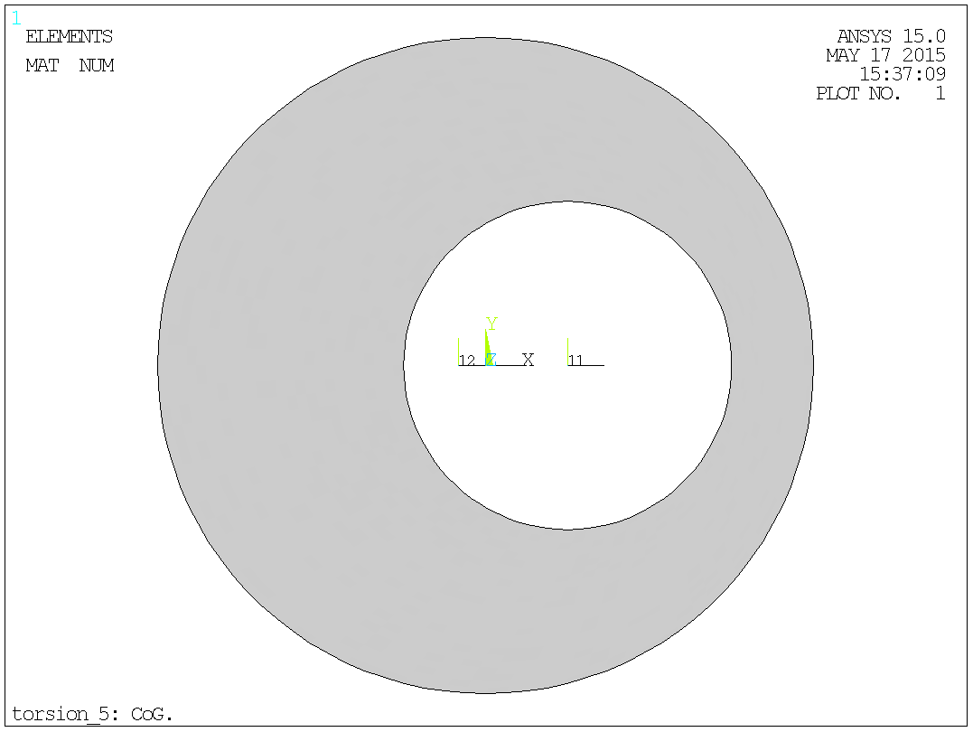
Fig. 7.4.1: The local coordinate system in CoG.
While still in the pre-processor, the boundary condition of the hole is defined. It's stated in the collection of formulas that, apart from the thermal analogy, a soap film (or membrane) analogy can be considered. The soap film spans a hole of the contour of the shaft and is subjected to a differential pressure. The height of the bubble corresponds to the potential and the gradient to the stress. The hole in the shaft can then be incorporated as a thin wire bent into the shape of the hole and floating at a constant elevation in the soap film. This explains why the hole must be modelled, meshed and loaded too - otherwise there would be a hole in the soap film. In the thermal analogy this must correspond to all nodes on the hole boundary has the same potential or temperature, thus the temperature must be coupled for these nodes:
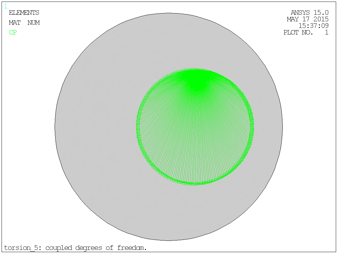
Fig. 7.5.1: Coupled degrees of freedom (temperature).
The support consists simply of defining a temperature of zero along the outer boundary of the cross-section:
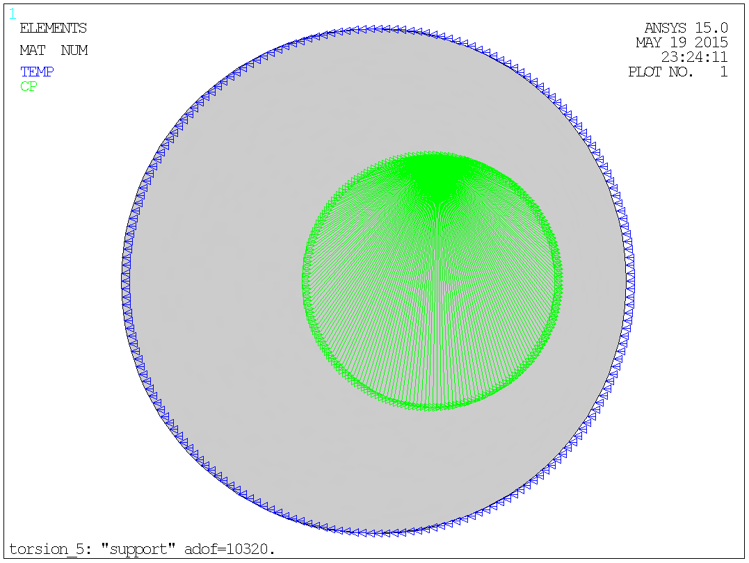
Fig. 7.6.1: Support (and cp's).
The number of active degrees of freedom will be reduced moderately, both by this support and the previous coupling of DoFs, (to 10320) but it's probably without importance.
Let the torque be 1.e+3 = 1 000 [Nmm].
As the formula for angular deflection of a circular bar is:
θr = (TL)/(IpG)
Where:
T ~ Torque.
L ~ Length.
Ip ~ Polar moment of inertia.
G ~ Shear modulus.
Then the expression for angular deflection of a circular bar pr. is unit length "twist" is:
θ = T/(IpG)
With:
T = 1.e+3 = 1000. [Nmm]. Given torque.
Ip = 22.5147 [mm4]. Polar moment of inertia as
described in § 7.4.
G = 78846. [N/mm2]. Shear modulus of steel as described in §
7.2.
The first guess on twist in the bar is the same as if the bar was circular - this is not the case, but it gives a first guess with some physical sense and a value that can have a reasonable size. Alternatively, a unit value could be used. In the end it should make no difference as the result of the initial load set will be scaled to obtain the correct final result.
The values below are only first guesses and will be designated by index 1.
The angular deflection of a circular steel bar pr. is unit length "twist" is:
θ1 = 1000/(22.5147·78846) = 0.5633183695E-03 [1/mm].
Heat generation pr. unit mass - according to the analogy, as described in § 2, the Heat generation pr. unit mass "q" is simply two times the twist:
q1 = 2·θ1 = 2·0.5633183695E-03 = 0.1126636739E-02
The heat generation is evenly distributed over cross-section:
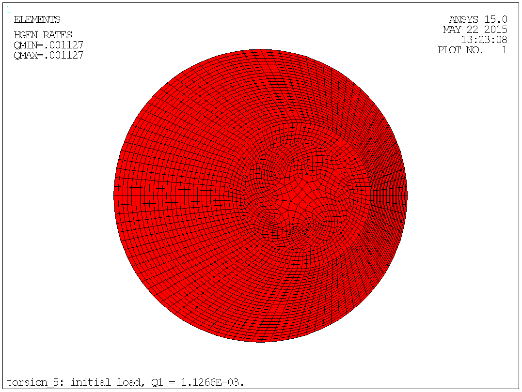
Fig. 7.7.1: Initial load.
The procedure is described in depth in § 4.
Solve the problem and go to the post-processor.
It's the initial (reaction) torque in the physical cross-section, that should be found, therefore select these elements. It's the thermal gradient in the radial (X) direction that's used:
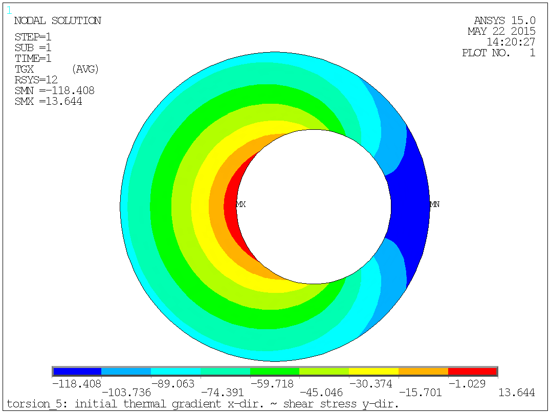
Fig. 7.8.1: Initial radial gradient.
The commands are:
csys,12 $ dsys,12 $ rsys,12 ! cyl. coord. sys. at centre of mass. etable,rcen,cent,x ! element centre radius. etable,tauy,tg,x ! therm. gradient, radial component. etable,area,volu ! volue (depth == 1) eq. area. smult,df,area,tauy ! tangential force pr. element. smult,dt,df,rcen ! torque pr. element. ssum ! all etable values are summed up. *get,name,ssum,dt ! torque from sum to parametre "name". trq1= -name ! torque in the shaft. |
And the output shows:
ACTIVE COORDINATE SYSTEM SET TO 12 (CYLINDRICAL) DISPLAY COORDINATE SYSTEM SET TO 12 (CYLINDRICAL) RSYS KEY SET TO 12 USE COORDINATE SYSTEM 12 FOR SOLUTION RESULTS STORE RCEN FROM ITEM=CENT COMP=X FOR ALL SELECTED ELEMENTS STORE TAUY FROM ITEM=TG COMP=X FOR ALL SELECTED ELEMENTS STORE AREA FROM ITEM=VOLU FOR ALL SELECTED ELEMENTS OPERATION SMUL RESULT= DF OPERAND1= AREA OPERAND2= TAUY FACTOR1= 1.0000 FACTOR2= 1.0000 CONSTANT= 0.0000 OPERATION SMUL RESULT= DT OPERAND1= DF OPERAND2= RCEN FACTOR1= 1.0000 FACTOR2= 1.0000 CONSTANT= 0.0000 SUM ALL THE ACTIVE ENTRIES IN THE ELEMENT TABLE TABLE LABEL TOTAL RCEN 3846.19 TAUY -164990. AREA 9.42478 DF -570.369 DT -948.573 *GET NAME AS SSUM DT VALUE= -948.5732 PARAMETER TRQ1 = 948.5731765 |
With the initial guess on the twist we obtained a torque of 948.573 [Nmm] but 1 000 [Nmm] was desired.
Return to the solution-module and perform a new analysis with the final load.
To find the final twist the initial twist shall be scaled to compensate for the deviation in torque. Obtained 948.573 [Nmm], desired 1 000 [Nmm]:
θ2 = θ1·1000/948.573 = 0.5633183695E-03·1000/948.573 = 0.5938586326E-03 [1/mm].
Heat generation pr. unit mass - according to the analogy, as described in § 2, the Heat generation pr. unit mass "q" is simply two times the twist:
q2 = 2·θ2 = 2·0.5938586326E-03 = 0.1187717265E-02.
The heat generation is evenly distributed over cross-section:
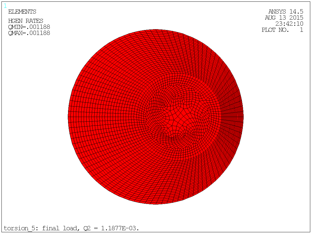
Fig. 7.9.1: Final load.
The procedure is described in depth in § 4.
Solve the problem and go to the post-processor.
It's the final (reaction) torque in the physical cross-section, that should be found, therefore select these elements. It's the thermal gradient in the radial (X) direction that's used:

Fig. 7.10.1: Final radial gradient.
The commands are:
csys,12 $ dsys,12 $ rsys,12 ! cyl. coord. sys. at centre of mass. etable,rcen,cent,x ! element centre radius. etable,tauy,tg,x ! therm. gradient, radial component. etable,area,volu ! volue (depth == 1) eq. area. smult,df,area,tauy ! tangential force pr. element. smult,dt,df,rcen ! torque pr. element. ssum ! all etable values are summed up. *get,name,ssum,dt ! torque from sum to parametre "name". trq2= -name ! torque in the shaft. |
And the output shows:
ACTIVE COORDINATE SYSTEM SET TO 12 (CYLINDRICAL) DISPLAY COORDINATE SYSTEM SET TO 12 (CYLINDRICAL) RSYS KEY SET TO 12 USE COORDINATE SYSTEM 12 FOR SOLUTION RESULTS STORE RCEN FROM ITEM=CENT COMP=X FOR ALL SELECTED ELEMENTS STORE TAUY FROM ITEM=TG COMP=X FOR ALL SELECTED ELEMENTS STORE AREA FROM ITEM=VOLU FOR ALL SELECTED ELEMENTS OPERATION SMUL RESULT= DF OPERAND1= AREA OPERAND2= TAUY FACTOR1= 1.0000 FACTOR2= 1.0000 CONSTANT= 0.0000 OPERATION SMUL RESULT= DT OPERAND1= DF OPERAND2= RCEN FACTOR1= 1.0000 FACTOR2= 1.0000 CONSTANT= 0.0000 SUM ALL THE ACTIVE ENTRIES IN THE ELEMENT TABLE TABLE LABEL TOTAL RCEN 3846.19 TAUY -173935. AREA 9.42478 DF -601.291 DT -1000.00 *GET NAME AS SSUM DT VALUE= -1000.000 PARAMETER TRQ2 = 999.9999997 |
With the final guess on the twist we are spot-on with the obtained torque!
With the general formula for angular deflection of a bar:
θr = (TL)/(KG)
Where:
T ~ Torque.
L ~ Length.
K ~ Stiffness.
G ~ Shear modulus.
By re-arranging the general formula K can be found to:
K = (TL)/(θrG) = T/(θG)
In this example the stiffness "the effective torsional moment of inertia" of the steel bar of a hollow circular cross-section of diameter Ø 4/2 and 0.5 [mm] eccentric is calculated to [mm4]:
K = T/(θG) = 1000/(0.5938586326E-03·78846) = 21.3568 [mm4]
The analytical solution says K = 21.3738 [mm4] a good agreement with the FEA value.
A plot of the temperature will give the "shape" of potential, first the solution of the full problem:
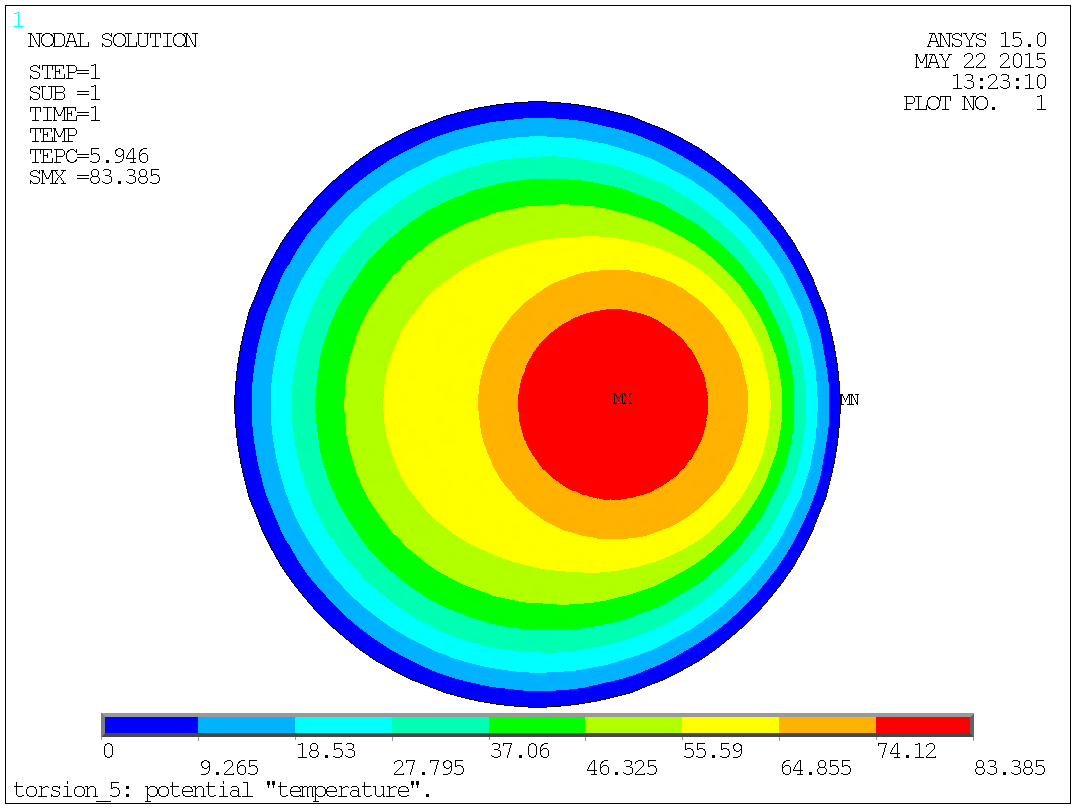
Fig. 7.12.1: The potential "temperature", full problem.
Then a plot of the temperature/potential, of the solid part of the shaft:
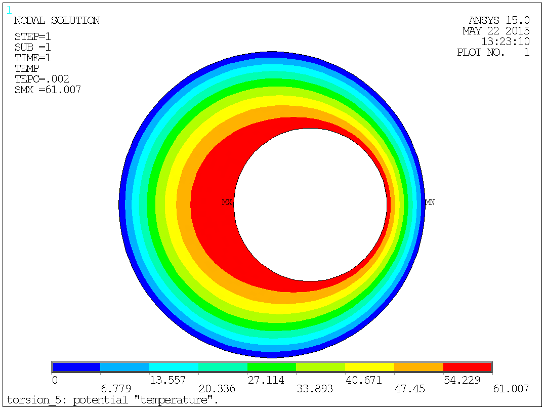
Fig. 7.12.2: The potential "temperature", solid part.
A plot of the thermal gradient will give the sear stress:
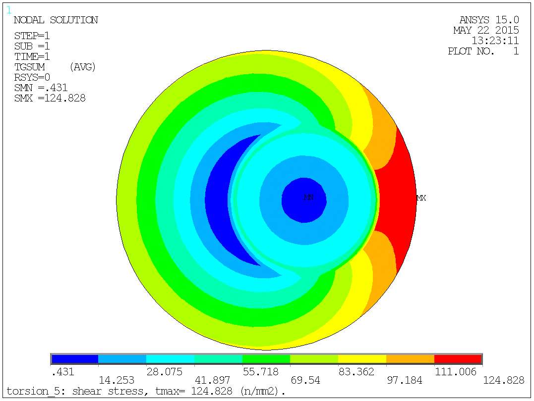
Fig. 7.12.3: The shear stress "thermal gradient", full problem.
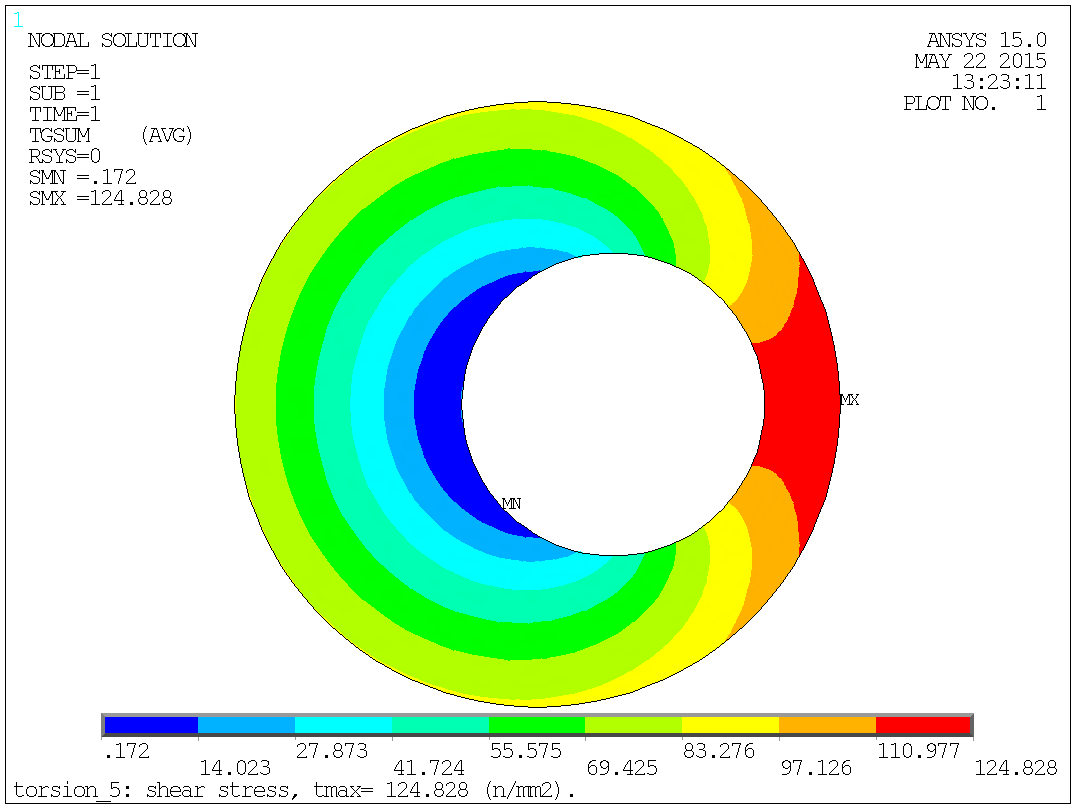
Fig. 7.12.4: The shear stress "thermal gradient", solid part.
Max shear stress can be read to: τ = 124.828 ~ 125. [N/mm2].
The max shear stress can finally be converted to an equivalent stress by the
traditionally used relationship, in this case:
σ = τ·√3 = 124.828·√3 = 216.208
~ 216. [N/mm2].
The analytical solution says τ = 122.287 [N/mm2] an o.k. agreement with the FEA value.
The iteration or better the scaling procedure can be shown as:
| Property | Symbol | Initial | Final | Formula |
|---|---|---|---|---|
| Initial stiffness | Ip | 22.5147 | ||
| Twist pr. unit length | θ | 0.563318 E-03 | 0.593859 E-03 | |
| Heat generation pr. unit mass | Q | 0.112664 E-02 | 0.118772 E-02 | |
| Torque | T | 948.573 | 1000.00 | 1000.00 |
| Max shear stress | τ | 118.408 | 124.827 | 122.287 |
| Stiffness | Keff | 21.3568 | 21.3568 | 21.3738 |
|
|
|
|
|
To illustrate the method, I've also chosen a maybe more common example of a thin-walled rectangular tube. The symmetry is used to ease modelling and reduce problem size.
The rectangular tube has the outer dimension of 200 × 100 [mm] and the wall thickness are respectively 5 and 10 [mm]:

Fig. 8.1.1: Full geometry.
A plot of the areas as modelled in ANSYS®. Both the solid part of the shaft and the hole are modelled - the hole must be meshed too, so it needs to be modelled (argument in § 7.5). The 4-fold symmetry is utilised to limit the model to ¼ of the full geometry:
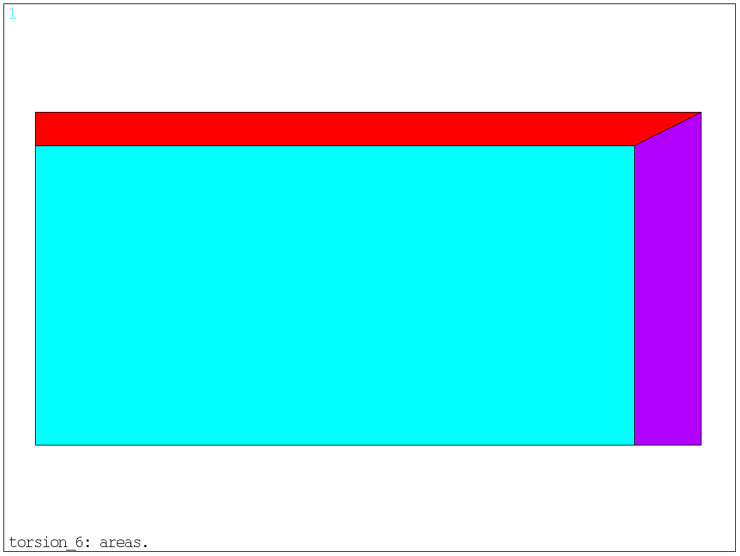
Fig. 8.1.2: Modelled areas.
The only material property needed is the heat conductivity. According to the analogy, as described in § 2, the heat conductivity "K" is simply the reciprocal of the shear modulus "G".
K = 1/G
If the specific value of the shear modulus isn't known the modulus of elasticity (Young's modulus) together with Poisson's ratio can be used as a basis. This will allow for consistent results if the results are compared with 3-D models.
G = E/(2(1+ν))
In a case with steel and units in N and mm, the values can be:
E = 205.e+3 [N/mm2].
ν = 0.3 [-].
G = E/(2(1+ν)) = (205.e+3)/(2(1+0.3)) = 78846. [N/mm2].
K = 1/G = 1/78846 = 0.1268292683E-04
Now if K is defined to this value in ANSYS®, so that the output shows:
PARAMETER K = 0.1268292683E-04 |
Then the command for the heat conductivity is:
mp,kxx,1,k |
And the output shows:
MATERIAL 1 KXX = 0.1268293E-04 |
In this example the areas are meshed with the quadrilateral element, no 77 - ANSYS® does a good job in meshing with quad's in 2-D, so why not use this element where ever possible, as quad's in general are better/more efficient than triangles. The hole is modelled too, and it must also be meshed (argument in § 7.5):
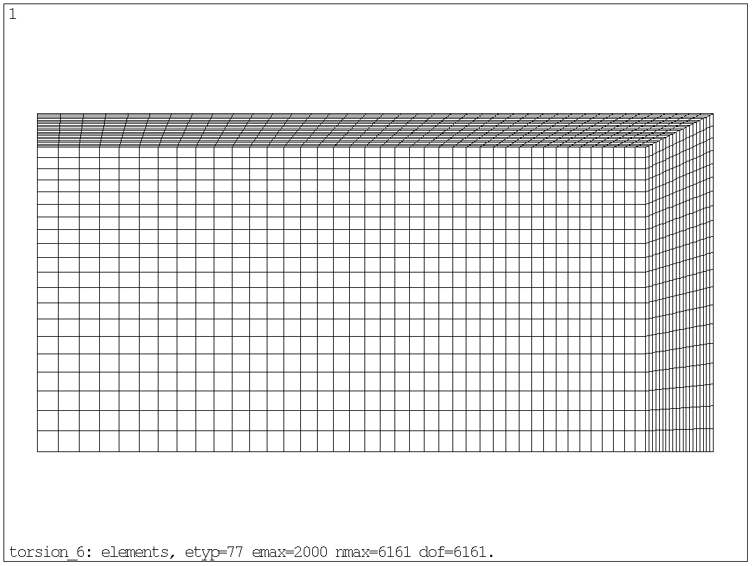
Fig. 8.3.1: Mesh.
The shown mesh, with element type 77, has 2000 elements, 6161 nodes and thereby also 6161 degrees of freedom. Though a relatively fine mesh still a small model.
Before leaving the pre-processor we can as well prepare load and torque calculation by issuing the "asum" command and extract polar moment of inertia. It's natural, and assumed here, that the geometry is modelled so, that the centre of the full geometry is positioned in the centre of the global coordinate system(s). "fold" = 4:
asum ! sum area properties. *get,name,area,,ior,z ! 1/4 polar moment of inertia. ip= name*fold ! total polar moment of inertia. |
And the output shows:
 PRINT GEOMETRY ITEMS ASSOCIATED WITH THE CURRENTLY SELECTED AREAS

 *** NOTE ***                            CP =       1.856   TIME= 11:06:38
 Density not associated with all selected areas.  Geometry items are
 based on a unit density.

   TOTAL NUMBER OF AREAS SELECTED =      2  (OUT OF      3 DEFINED)

   TOTAL SURFACE AREA OF ALL SELECTED AREAS =   950.00

   TOTAL VOLUME OF ALL SELECTED AREAS =   950.00

   CENTER OF MASS:  XC=  71.316      YC=  35.658      ZC=  0.0000

                     *** MOMENTS OF INERTIA ***
           (BASED ON A UNIT DENSITY AND A UNIT THICKNESS)

         ABOUT ORIGIN     ABOUT CENTER OF MASS    PRINCIPAL
     IXX =   0.14329E+07       0.22501E+06       0.13251E+06
     IYY =   0.57317E+07       0.90002E+06       0.99252E+06
     IZZ =   0.71646E+07       0.11250E+07       0.11250E+07
     IXY =  -0.21494E+07       0.26645E+06
     IYZ =    0.0000            0.0000
     IZX =    0.0000            0.0000

     PRINCIPAL ORIENTATION VECTORS (X,Y,Z):
       0.945 -0.328  0.000    0.328  0.945  0.000    0.000  0.000  1.000
       (THXY=  -19.145  THYZ=    0.000  THZX=    0.000)

 *GET  NAME      FROM  AREA  ITEM=IOR  Z     VALUE=  7164583.33

 PARAMETER IP =     28658333.33
|
While still in the pre-processor, the boundary condition of the hole is defined. Temperature must be coupled for these nodes (argument in § 7.5):
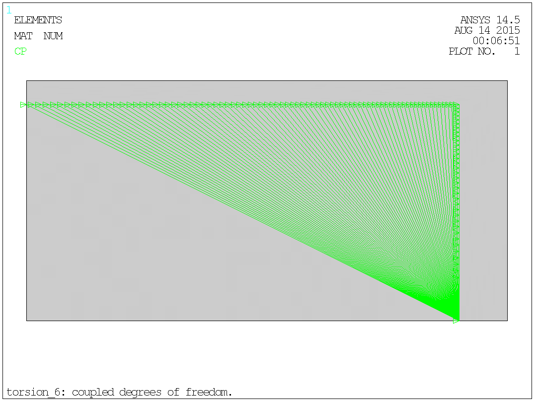
Fig. 8.5.1: Coupled degrees of freedom (temperature).
The support consists simply of defining a temperature of zero along the outer boundary of the cross-section:
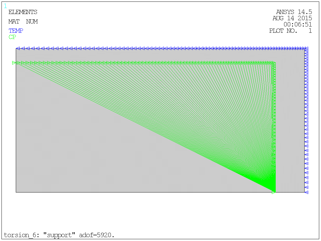
Fig. 8.6.1: Support (and cp's).
The number of active degrees of freedom will be reduced moderately, both by this support and the previous coupling of DoFs, (to 5920) but it's probably without importance.
Let the torque be 10.e+6 = 10 000 000 [Nmm].
As the formula for angular deflection of a circular bar is:
θr = (TL)/(IpG)
Where:
T ~ Torque.
L ~ Length.
Ip ~ Polar moment of inertia.
G ~ Shear modulus.
Then the expression for angular deflection of a circular bar pr. is unit length "twist" is:
θ = T/(IpG)
With:
T = 10.e+6 = 10 000 000 [Nmm]. Given torque.
Ip = 28 658 333 [mm4]. Polar moment of inertia as
described in § 8.4.
G = 78846. [N/mm2]. Shear modulus of steel as described in
§ 8.2.
The first guess on twist in the bar is the same as if the bar was circular - this is not the case, but it gives a first guess with some physical sense and a value that can have a reasonable size. Alternatively, a unit value could be used. In the end it should make no difference as the result of the initial load set will be scaled to obtain the correct final result.
The values below are only first guesses and will be designated by index 1.
The angular deflection of a circular steel bar pr. is unit length "twist" is:
θ1 = 10000000/(28658333·78846) = 0.4425563302E-05 [1/mm].
Heat generation pr. unit mass - according to the analogy, as described in § 2, the Heat generation pr. unit mass "q" is simply two times the twist:
q1 = 2·θ1 = 2·0.4425563302E-05 = 0.8851126604E-05
The heat generation is evenly distributed over cross-section, incl. the hole:
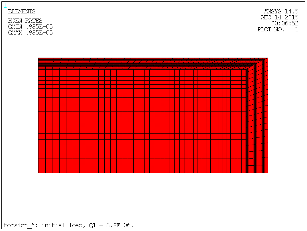
Fig. 8.7.1: Initial load.
The procedure is described in depth in § 4.
Solve the problem and go to the post-processor.
It's the initial (reaction) torque in the physical cross-section, that should be found, therefore select these elements. It's the radial (X-dir.) thermal gradient corresponding to the tangential (Y-dir.) shear stress that's used:
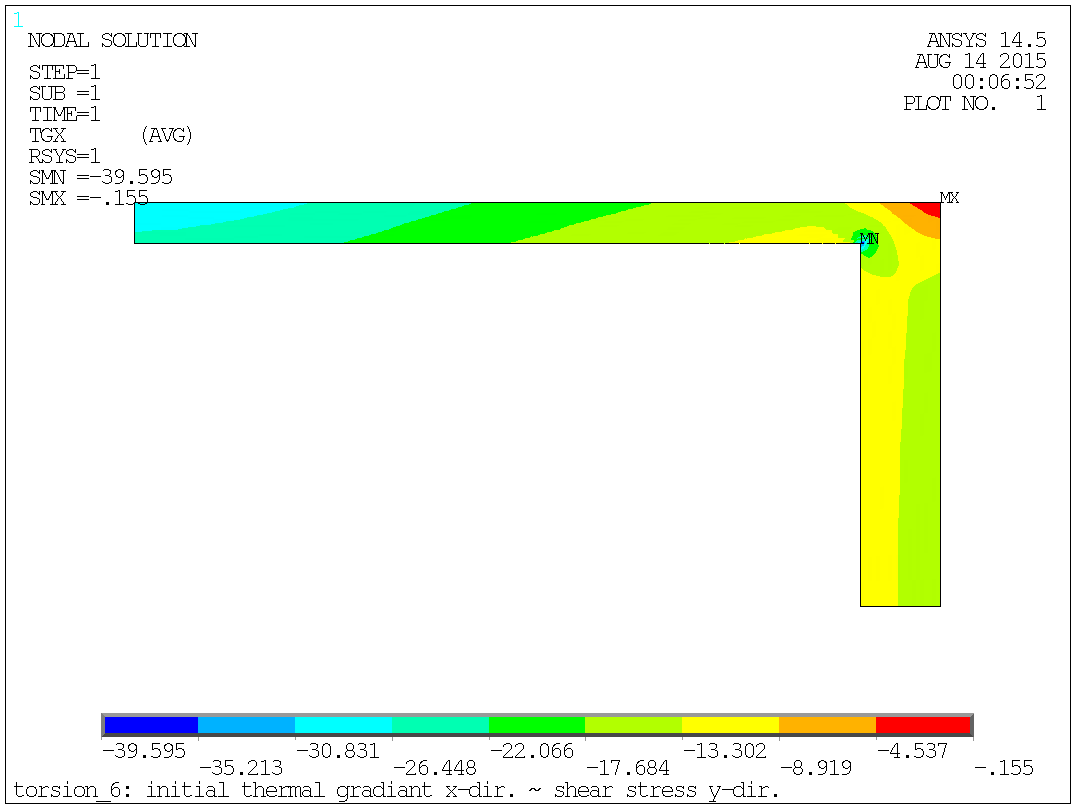
Fig. 8.8.1: Initial radial gradient.
The commands are (fold = 4):
csys,1 $ dsys,1 $ rsys,1 ! cyl. coord. sys. etable,rcen,cent,x ! element centre radius. etable,tauy,tg,x ! therm. gradient, radial component. etable,area,volu ! volue (depth == 1) eq. area. smult,df,area,tauy ! tangential force pr. element. smult,dt,df,rcen ! torque pr. element. ssum ! all etable values are summed up. *get,name,ssum,dt ! torque from sum to parametre "name". trq1= -name*fold ! torque in the shaft. |
And the output shows:
ACTIVE COORDINATE SYSTEM SET TO 1 (CYLINDRICAL) Z- CYL. AXIS DISPLAY COORDINATE SYSTEM SET TO 1 (CYLINDRICAL) RSYS KEY SET TO 1 USE COORDINATE SYSTEM 1 FOR SOLUTION RESULTS STORE RCEN FROM ITEM=CENT COMP=X FOR ALL SELECTED ELEMENTS STORE TAUY FROM ITEM=TG COMP=X FOR ALL SELECTED ELEMENTS STORE AREA FROM ITEM=VOLU FOR ALL SELECTED ELEMENTS OPERATION SMUL RESULT= DF OPERAND1= AREA OPERAND2= TAUY FACTOR1= 1.0000 FACTOR2= 1.0000 CONSTANT= 0.0000 OPERATION SMUL RESULT= DT OPERAND1= DF OPERAND2= RCEN FACTOR1= 1.0000 FACTOR2= 1.0000 CONSTANT= 0.0000 SUM ALL THE ACTIVE ENTRIES IN THE ELEMENT TABLE TABLE LABEL TOTAL RCEN 99006.9 TAUY -20083.6 AREA 950.000 DF -15538.7 DT -0.122991E+07 *GET NAME AS SSUM DT VALUE= -1229913. PARAMETER TRQ1 = 4919650.330 |
With the initial guess on the twist we obtained a torque of 4 918 274 [Nmm] but 10 000 000 [Nmm] was desired.
Return to the solution-module and perform a new analysis with the final load.
To find the final twist the initial twist shall be scaled to compensate for the deviation in torque. Obtained 4 918 274 [Nmm], desired 10 000 000 [Nmm]:
θ2 = θ1·10000000/4918274 = 0.4425563302E-05·10000000/4919650 = 0.8995686695E-05 [1/mm].
Heat generation pr. unit mass - according to the analogy, as described in § 2, the Heat generation pr. unit mass "q" is simply two times the twist:
q2 = 2·θ2 = 2·0.8995686695E-05 = 0.1799137339E-04.
The heat generation is evenly distributed over cross-section:
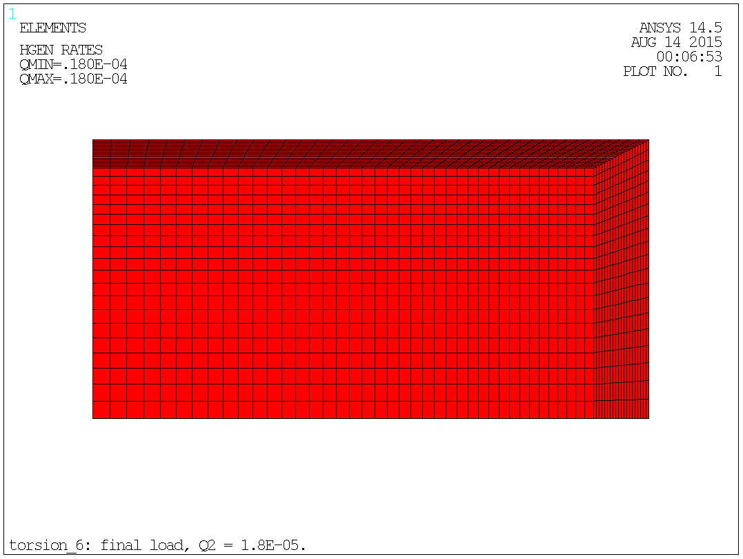
Fig. 8.9.1: Final load.
The procedure is described in depth in § 4.
Solve the problem and go to the post-processor.
It's the initial (reaction) torque in the physical cross-section, that should be found, therefore select these elements. It's the radial (X-dir.) thermal gradient corresponding to the tangential (Y-dir.) shear stress that's used:

Fig. 8.10.1: Final radial gradient.
The commands are (fold = 4):
csys,1 $ dsys,1 $ rsys,1 ! cyl. coord. sys. etable,rcen,cent,x ! element centre radius. etable,tauy,tg,x ! therm. gradient, radial component. etable,area,volu ! volue (depth == 1) eq. area. smult,df,area,tauy ! tangential force pr. element. smult,dt,df,rcen ! torque pr. element. ssum ! all etable values are summed up. *get,name,ssum,dt ! torque from sum to parametre "name". trq2= -name*fold ! torque in the shaft. |
And the output shows:
ACTIVE COORDINATE SYSTEM SET TO 1 (CYLINDRICAL) Z- CYL. AXIS DISPLAY COORDINATE SYSTEM SET TO 1 (CYLINDRICAL) RSYS KEY SET TO 1 USE COORDINATE SYSTEM 1 FOR SOLUTION RESULTS STORE RCEN FROM ITEM=CENT COMP=X FOR ALL SELECTED ELEMENTS STORE TAUY FROM ITEM=TG COMP=X FOR ALL SELECTED ELEMENTS STORE AREA FROM ITEM=VOLU FOR ALL SELECTED ELEMENTS OPERATION SMUL RESULT= DF OPERAND1= AREA OPERAND2= TAUY FACTOR1= 1.0000 FACTOR2= 1.0000 CONSTANT= 0.0000 OPERATION SMUL RESULT= DT OPERAND1= DF OPERAND2= RCEN FACTOR1= 1.0000 FACTOR2= 1.0000 CONSTANT= 0.0000 SUM ALL THE ACTIVE ENTRIES IN THE ELEMENT TABLE TABLE LABEL TOTAL RCEN 99006.9 TAUY -40823.2 AREA 950.000 DF -31585.1 DT -0.250000E+07 *GET NAME AS SSUM DT VALUE= -2500000. PARAMETER TRQ2 = 9999999.996 |
With the final guess on the twist we are spot-on with the obtained torque!
With the general formula for angular deflection of a bar:
θr = (TL)/(KG)
Where:
T ~ Torque.
L ~ Length.
K ~ Stiffness.
G ~ Shear modulus.
By re-arranging the general formula K can be found to:
K = (TL)/(θrG) = T/(θG)
In this example the stiffness "the effective torsional moment of inertia" of the rectangular tube with the outer dimension of 200 × 100 [mm] and the wall thickness of respectively 5 and 10 [mm] is calculated to [mm4]:
K = T/(θG) = 10000000/(0.8995686695E-05·78846) = 14 098 898. [mm4]
The analytical solution says K = 13 718 000 [mm4] a quite good agreement with the FEA value.
A plot of the temperature will give the "shape" of potential, first the solution of the full problem:
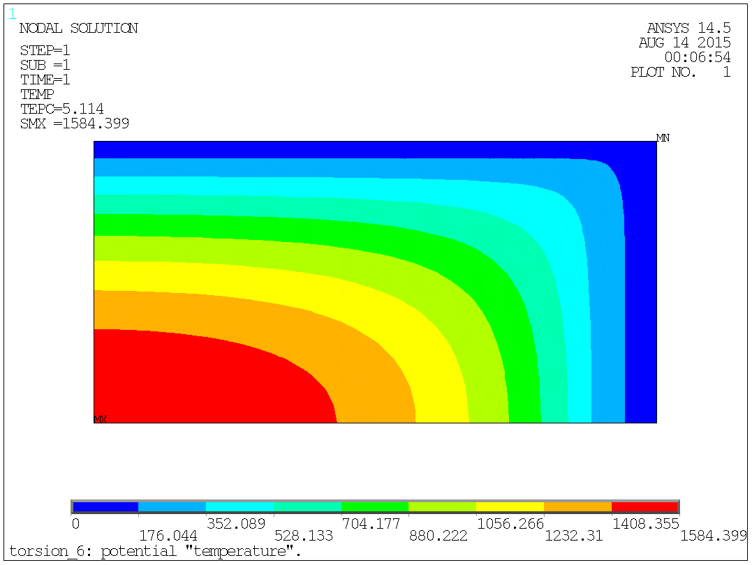
Fig. 8.12.1: The potential "temperature", full problem.
Then a plot of the temperature/potential, of the solid part of the tube:
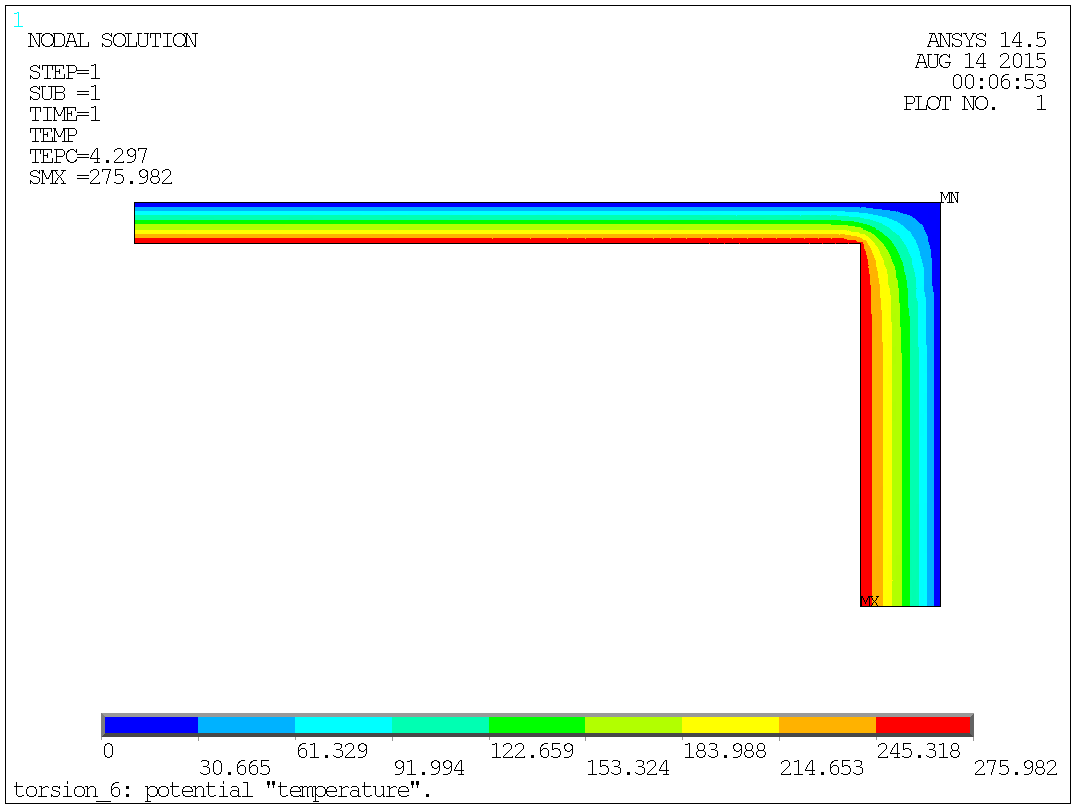
Fig. 8.12.2: The potential "temperature", solid part.
A plot of the thermal gradient will give the sear stress:

Fig. 8.12.3: The shear stress "thermal gradient", full problem.
Only stresses in the physical part of the structure is relevant:
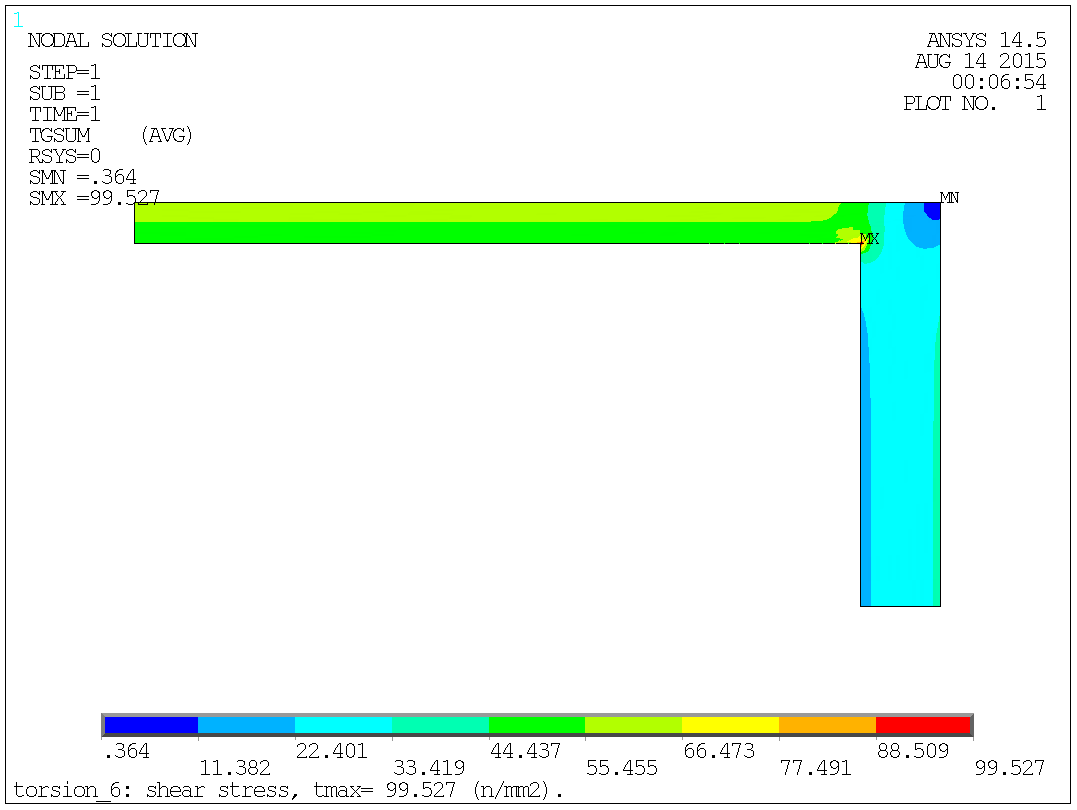
Fig. 8.12.4: The shear stress "thermal gradient", solid part.
Max shear stress can be read to: τ = 99.527 ~ 100. [N/mm2] but this value hasn't much meaning as it represents a singularity and will grow to infinite values with increasing mesh density - as predicted by the collection of formulas. The information about the stress concentration located here is however important.
The stress at the centre line of the long, thin side:
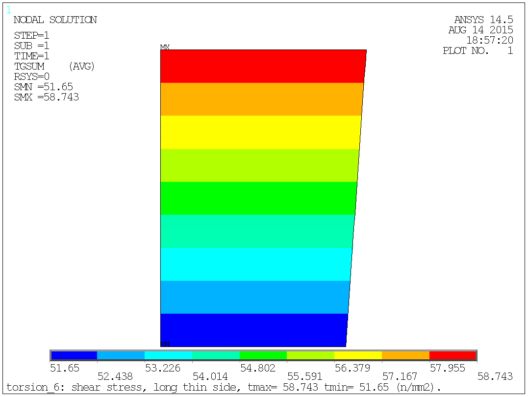
Fig. 8.12.5: The shear stress at the centre line of the long, thin side.
The stress at the centre line of the short, thick side:
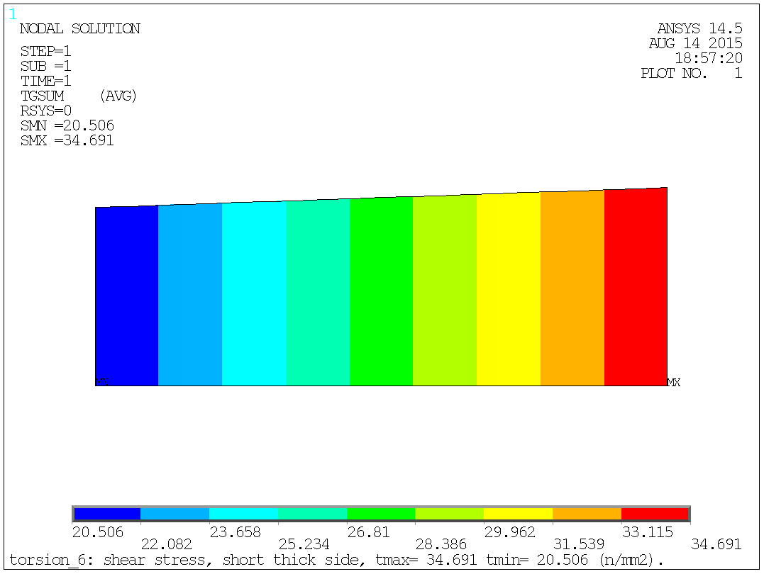
Fig. 8.12.6: The shear stress "thermal gradient", solid part.
The stress distribution across the centre lines of the two sides are effectively linear and a mean stress can well be found as the average between max and min values:
Long, thin side:
τavg = (58.743 + 51.65)/2 = 55.2, formula: 57.0
Short, thick side:
τavg = (34.691 + 20.506)/2 = 27.6, formula: 28.5
Good agreement between FEA values and formula.
The iteration or better the scaling procedure can be shown as:
| Property | Symbol | Initial | Final | Formula |
|---|---|---|---|---|
| Initial stiffness | Ip | 28658333. | ||
| Twist pr. unit length | θ | 0.442556 E-05 | 0.899569 E-05 | |
| Heat generation pr. unit mass | Q | 0.885113 E-05 | 0.179914 E-04 | |
| Torque | T | 4919650. | 10000000. | 10000000. |
| Max shear stress, thin side | τa | 27.1547 | 55.1965 | 56.9801 |
| Max shear stress, thick side | τb | 13.5775 | 27.5985 | 28.4900 |
| Stiffness | Keff | 14098898. | 14098898. | 13718000. |
The similarity of ideal flow can be recognised in fig. 8.12.1 and fig. 8.12.2
above. As a consequence, the product of mean shear stress (mean flow) and side
width must be the same on the two sides (formula values):
τa · ta = 56.9801 · 5 = 284.905
τb · tb = 28.4900 · 10 = 284.900
The same exercise with the FEA values says:
τa · ta = 55.1965 · 5 = 275.983
τb · tb = 27.5985 · 10 = 275.985
The singularity in the stress plot in the above section, fig. 8.12.4 can be eliminated by a rather large inner radius. This is only good common sense and mentioned in the collection of formulas.
Shown below an inner corner with a radius of 9 [mm]. A radius of this size moves the location of max stress away from the corner and to the straight, outer side of the thin side:
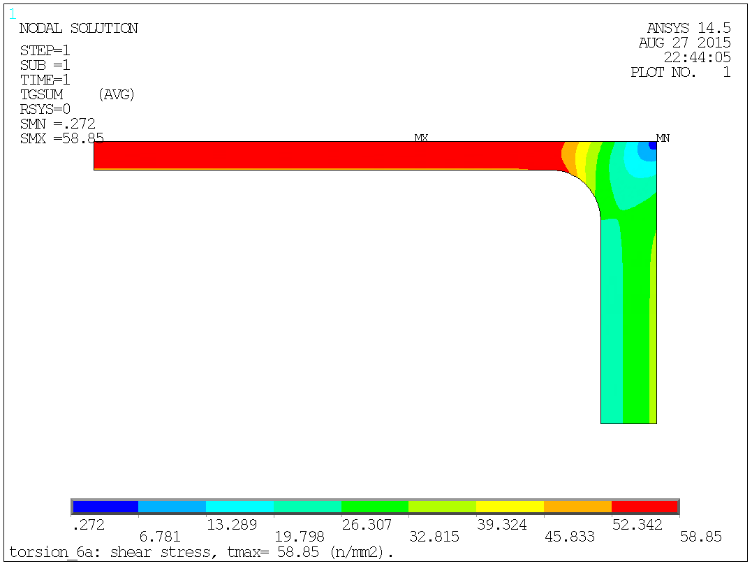
Fig. 8.13.1: The shear stress "thermal gradient", solid part.
As shown in § 6.11, the plot can be expanded to show the full geometry. The command used for the expansion here is:
/expand,1,rect,half,0,1.e-4,0,1,rect,half,1.e-4,0,0 |
The stress plot of the full cross-section of the tube will then look like:
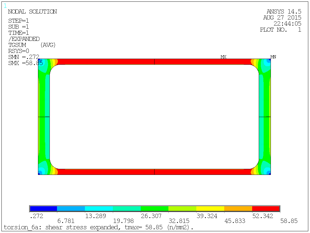
Fig. 8.13.2: The shear stress "thermal gradient", full cross-section.
|
|
|
|
|
| Overview |